Information Spaces for Mobile Robots - LaValle

Information Spaces for Mobile Robots Benjam´ın Tovar

Anna Yershova Jason M. O’Kane Steven M. LaValle Dept. of Computer Science University of Illinois Urbana-Champaign, IL 61801. USA {btovar,yershova,jokane,lavalle}@uiuc.edu

Abstract Planning with sensing uncertainty is central to robotics. Sensor limitations often prevent accurate state estimation of the robot. Two general approaches can be taken for solving robotics tasks given sensing uncertainty. The first approach is to estimate the state and to solve the given task using the estimate as the real state. However, estimation of the state may sometimes be harder than solving the original task. The other approach is to avoid estimation of the state, which can be achieved by defining the information space, the space of all histories of actions and sensing observations of a robot system. Considering information spaces brings better understanding of problems involving uncertainty, and also allows finding better solutions to such problems. In this paper we give a brief description of the information space framework, followed by its use in some robotic tasks.

1

Introduction

Often robots have to plan and execute tasks while being uncertain about their configuration and the environment in which they are acting. From a robotic perspective, the state of a robot system, or simply the state, represents the information that together with the control input, fully specifies the situation of the robot system. It refers to the position in space, velocities in joints or wheels, levels of energy consumption, the environment in which the robot is in, etc. Classical approaches for robot planning assume a perfect knowledge of the robot state. Such perfect knowledge is virtually unattainable, given noisy readings from the available sensors and limitations on the number of sensors the robot can have. Therefore, some crucial information may simply be unavailable to the robot (for example, the information about the orientation is not available to the robot without a compass). Therefore, many research efforts have

been focused on the estimation of the state. If such estimations are reliable, they can be considered as the true robot state, forgetting that there is uncertainty in the state information. In control theory, for example, the concept of an observer is well understood [2], and if the observer converges sufficiently fast, the value of the state variables of the observer is taken as the value of the state variables of the system. In mobile robotics, simultaneous localization and mapping (SLAM) approaches have received considerable attention in recent years [3, 21]. The goal of the SLAM approaches is to correctly estimate the current state of the robot. However, an interesting approach is to avoid the state estimation all together. In fact, the necessity for the knowledge of the robot state can be considered as an artifact of a planning algorithm. While knowing the state of the robot is sufficient to solve a task, it may not be necessary. In other words, a robot may not know its current state, and still be able to solve a specific task. It has been shown in numerous robotics works that robots can efficiently solve complicated tasks with no estimation of its current state. Much of the early work in this direction was in the context of object manipulation [9, 20]. Other work includes information invariants [5], sensor design [8], bug algorithms for navigation [19, 13], robot localization [6], POMDPs [16], and error detection and recovery [4]. All of these works present seemingly different approaches for solving given robotics tasks. In this paper we describe a framework based on information spaces that generalizes planning strategies for robotic systems with sensing uncertainty. For this we first formulate the general planning problem presented to the robot. This usually includes: the state space, i.e. the set of states of the robotic system (robot and environment); the action space, i.e. the set of actions that the robot can perform; the observation space, i.e. the set of observations that is available to the robot from sensors; sensor mappings, which produce an observation for each state of the robot; state transition function, which produces

a state for each action; and the goal, which is expressed in terms of the histories of actions and observations. Planning problems with sensing uncertainty are naturally expressed in terms of information states, and the space where they live, the information space. In this paper we explore some results for robot planning in the information space framework. There are many exciting open research problems with information spaces. It is our hope that this paper will stimulate further research in analyzing the information spaces for robotics systems and bring more efficient strategies for solving robotics tasks.

2

Preliminaries

In the following discussion, let X be a set called the state space, and let U (x) the set of actions available to the robot from state x ∈ X. At each stage k, it is assumed that a nature action θk is chosen from a set Θ(xk , uk ), given the current state of the robot xk ∈ X, and the action executed uk ∈ U (xk ). The role of Θ(xk , uk ) is to model events the robot cannot control. For example, it can model control execution inaccuracies, unpredictable changes in a dynamic environment, etc. Let f be the state transition equation, that produces a state, f (x, u, θ) for every x ∈ X, u ∈ U and θ ∈ Θ(x, u). Note that f is not known for every planning problem. For simplicity of presentation, we assume that time is discrete. The continuous time case is developed in [17]. For a more extensive description see [17, 23]. A robot may retrieve information regarding its state from three sources: 1. Initial conditions. The initial conditions refer to all the information the robot is given prior to the planning task. For example, the initial state x1 ∈ X may be given, or the initial state may lie in a given subset X1 ⊂ X. Also, the initial state may follow a given probability distribution P (x1 ) over X. Note that the calibration of a robotic system is considered in the previous cases. If all the state variables are calibrated, then the initial state is known. On the contrary, if only some state variables are calibrated, this correspond to the case when a subset X1 is given. The initial conditions will be denoted with η0 . 2. Sensor observations. A sensor is a device that provides some measurement of the current state. Thus, a sensor observation provides measurements of the state during execution. Formally, let Y denote the observation space, and let h denote a sensor mapping. If given the state, the observation

is completely determined, then h takes the form h : X → Y . Another important case is when nature interferes with the observation. In this case the mapping takes the form y = h(x, φ) ∈ Y , with φ ∈ Φ, in which Φ(x) is the set of nature sensing actions defined for each x ∈ X. Finally, the observation may also depend on previous states, in which the mapping for the k observation takes the form yk = h(x1 , ..., xk , φk ). 3. Actions executed. An action executed may provide valuable information regarding the robot state. For example, in the absence of control errors, if the robot is commanded to move one meter east, it is known that the robot is now one meter further east than before.

2.1

The information space

The information available to the robot when the plan is at stage k should be determined either from the new observations, or the accumulation of previous information. It is assumed that the robot keeps a record of each of the observations made. Thus, the observation history, y˜ = (y1 , y2 , ..., yk ), is the ordered sequence of observations up to stage k. Similarly, the action history, u ˜ = (u1 , u2 , ..., uk−1 ), is the record of the actions taken. It runs until k −1, because action uk−1 is applied in state xk−1 , to yield the current state xk , where the observation yk is made. The information state at stage k is defined as ηk = (η0 , u ˜k−1 , y˜k ), that is, the initial condition together with the history. Alternatively, an information state can be expressed recursively as ηk = (ηk−1 , uk−1 , yk ), because the difference between the previous and the current information state consists of the new observation made and the new action taken. The set of all possible information states is called the information space, I. Usually we do not deal with I directly, given that the size of an information state grows linearly with the number of stages, and this becomes intractable very fast. Thus, we have to look for methods that collapse the information space. One simple method for collapsing the information space is based on the inferences that can be done given an information state. If the information state ηk is available, it is possible to compute the set Xk (ηk ) ⊂ X in which the actual xk is known to lie. The set Xk (ηk ) is called a derived information state. To

compute the derived information state, we have to integrate the observations and actions performed. Given an observation, we can find the set of all possible states the robot may be in that are congruent with the observation: H(y) = {x | y = h(x, ψ), for ψ ∈ Ψ(x)}. The set H(y) is called the preimage of y. Similarly, if we let the actions available depend on the current state, the robot can determine a set of states W where it may be: W (Uk ) = {x′ | Uk = U (x′ ) for x′ ∈ X}, in which Uk are the actions available at stage k. The current state then lies in the set H ∩ W . Note, however, that it can be assumed that the robot has some kind of sensor that detects which kind of actions are available. This reduces the computation of W and H into only the computation of H. Thus, only the case when U is fixed for all x ∈ X is important. From the state transition equation, it is possible to know which states may be reached if action u is applied at state x. Let F be this set, formally defined as F (x, u) = {x′ ∈ X | ∃θ ∈ Θ(x, u) for which x′ = f (x, u, θ)}. If we further assume that X is countably infinite, the derived information state Xk (ηk ) can be computed using induction. Note that F and H eliminate the direct appearance of nature actions. The base case (k = 1) of the induction is X1 = η0 ∩ H(y1 ). This first step consists only of making the initial condition consistent with the first observation. Now assume inductively that Xk (ηk ) ⊆ X is available, and Xk+1 (ηk+1 ) should be computed. First note that ηk+1 = (ηk , uk , yk+1 ), and the new information is provided only by uk and yk+1 . It is known that the state lies anywhere in H(yk+1 ), On the other hand, if xk was known, after applying uk , the state lies somewhere in F (xk , uk ). Since xk is unknown, but it is known that xk ∈ Xk (ηk ), the new derived information state is Xk+1 (ηk , uk , yk+1 ) =

[

F (xk , uk ) ∩ H(yk+1 ).

xk ∈Xk (ηk )

Given that the derived information state is always a subset of X, the derived information space denoted by

I ◦ , can be defined as I ◦ = 2X . Note that if X is finite, I ◦ is also finite, which makes it preferable if the number of stages is much larger than the size of X. The derived information space developed until now is nondeterministic. Derived information spaces can be obtained also from probabilities distributions. Examples of such spaces are presented in Section 3.5, and are described extensively in [17].

3

Examples of Information Spaces

In this section we present several examples in which the state is unknown, and the concept of information space comes naturally. We do not intent to give a full range of applications, rather, the examples are drawn from our previous work instead. As we said in the introduction, we hope for an increased interest in information spaces, since they offer an exciting point of view from which robotic problems can be solved.

3.1

Visibility-based pursuit-evasion

In the pursuit-evasion problem, a robot, called the pursuer, has to move in such a way that it could find another robot, called the evader. In a complete antagonistic setting, the evader does not want to be found, and can move arbitrarily fast compared to the pursuer. Assume that the pursuer has a map of the environment, and it is perfectly localized with respect to this map. How should the pursuer plan its movements in order to find all of the evaders? The answer depends on which sensors are available to the pursuer. Since the pursuer does not know where the evaders are, we can provide the pursuer with an ideal sensor called the evader locator, which when used, will tell the location of the evaders to the pursuer. While this is a valid formulation of the pursuit-evasion problem, its solution is trivial, given that we provided the pursuer with perfect information of the state of the task. Thus, a more interesting formulation considers providing the robot with sensors that report robot only local information. For example, providing the pursuer with a camera, can only tell weather an evader is present in the current visible region, or not. This version of the pursuit-evasion problem was presented in [10], and we describe it here from the information space framework. Formally, assume that the pursuer moves in a connected open set R ⊂ R2 . The boundary, ∂R, of R is assumed to be polygonal and simply-connected. The evader is modeled as a moving point in R. The evader position e(t) at time t is determined by a continuous position function e : [0, ∞) → R. The pursuer is also modeled

E? Wall Wall

E? Wall

P

E?

E? E?

E? Wall

(a)

Wall

Wall

(b)

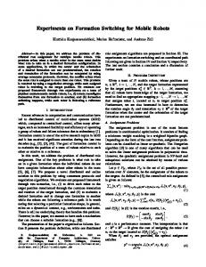
Figure 1: Each shadow region is a portion of the environment that may or may not contain the evader.

as a point, with position p(t). The pursuer has an exact geometric representation of R, and it is perfectly localized with respect to R. The pursuer also has a visibility sensor, which returns the visibility region from its current position. For a point q ∈ R, the visibility region W (q) includes all the points in R that can be joined with q through a line segment without intersecting δR. The task is to find a path p : [0, 1] → R for the pursuer such that the evader is guaranteed to be detected, regardless of its position function e(t), which is unknown to the pursuer. The state yields the position of the pursuer and evader, x = (p, e), which results in the state space X ⊂ R2 × R2 = R4 . Since the position of the evader is unknown, the state is unknown. The observation space Y , is a collection of subsets of R. For each q ∈ R, the sensor yields a visibility polygon W (p) ⊂ R. Consider the information state at time t. For the initial condition, p(0) is given and the evader may lie anywhere in R. The input history u ˜t , can be expressed as the position function of the pursuer. Thus, the information state is defined as:

shadow region disappears, it means that the given region is now visible to the pursuer, and thus does not contain the evader. Also, if a contaminated region merges with a cleared one, the new region should be labeled contaminated, and so on. The visual events induce a decomposition of R, called the aspect graph [14], or the visibility-cell decomposition [11]. In these decompositions, if the robot moves inside a cell there is no significant change in information. The robot receives roughly the same information from the sensors. Such movements are called conservative in the sense that they preserve the current robot’s information. In contrast, when the robot crosses one of the cells’ boundary edges, the structure of the visibility region suffers a drastic change, and the robot’s information may be modified [7]. In these case there are two kinds of visual events. One kind is triggered when the robot crosses an environment’s boundary generalized inflection ray, and the other when it crosses the complement of bitangent line segments of the boundary. An inflection is a change in the sign of the curvature of the environment’s boundary. We use the term “generalized,” as in [18], to include polygonal boundaries. Given a generalized inflection, an inflection ray is found by extending a ray from the inflection until it hits another point of the environment’s boundary. A bitangent line segment is a segment completely contained in the environment representation, whose supporting line is tangent to two points of the boundary, and whose endpoints are these points of tangency. A common general position assumption is that no line is tangent to more than two points of the boundary (thus the term bitangent). For each bitangent, its complement is found by extending outward from each point of tangency until the environment’s boundary is hit again (see Figure 3).

ηt = ((p(0), R), p(t), y˜t ). Since the pursuer position is always known, the interesting part is the subset of R in which the evader may lie. Thus, the derived information state can be expressed as Xt (ηt ) = (p(t), E(ηt )), in which E(ηt )) is the smallest subset of R that is known to contain the evader, given ηt . The visibility region divides R in several shadow regions, which are regions that are not visible to the robot (Figure 1). When the evader may be hidden in one of these regions, the region is said to be contaminated, otherwise it is said to be cleared. As the pursuer moves, the shadow regions appear, disappear, merge or split. Such events, called visual events, are produced by combinatorial changes in the visibility region. The visual events provide the only way to vary E(ηt ). For example, if a

With this decomposition we can collapse the information space even further. It was proved [11] that each of the cells produced is convex. Thus, if the pursuer is inside a cell, it can detect if the evader is also inside or not. Furthermore, it can compute which cells are cleared, or become recontaminated when moving from one cell to the other. The state space is now discrete, because the exact positions of the pursuer and evader are not relevant anymore; only matters whether or not they are inside of a given cell. We can encode E(ηk ) as binary vector, with a label for each cell indicating weather it is cleared. With this, the solution plan p(t) can be found using a simple search in the derived information space [10].

3.2

Visibility-based tasks with Gap Navigation Trees

far

R

b near far

In the previous example, in principle, the planning strategy used the exact geometry of both visibility regions and the environment. However, we are interested in such information as an intermediate product, since it is only important weather a certain region is cleared, or weather it becomes recontaminated by merging with other regions. Thus, we are not interested in the exact description of the visibility regions, but in how they change. As presented in [12, 26, 27], we can further collapse the information space by designing a sensor that detects the combinatorial changes in the visibility region. Furthermore, we can eliminate the need of a map, and the robot can solve some visibility-based tasks in unknown environments. A visibility region is bounded of edges completely contained in the environment boundary, and by edges collinear with the position of the robot. The later are called spurious edges. When a spurious edge either appears, disappears, splits or merges, a combinatorial change in the visibility region occurs. From the robot’s perspective, the spurious edges are the discontinuities in depth information in the environment. Note that geometric information of the spurious edges is not relevant for the visual event detection. The events will be the same in spite of the exact length and angular position of the spurious edges. Their order is relevant, however, because we are interested in which discontinuity disappeared, or merged with another, for example. Although the precise distances to the walls may be unknown, the robot only needs an edge detector that can detect each of the discontinuities, and return their order relative to the robot’s heading. Each of this discontinuities is referred to as a gap, and the sensor as a gap sensor [24]. As shown in [27, 12, 26], a robot using a gap sensor, with no other sensing ability assumed (it has neither a compass nor a reliable odometer) can compute shortestpaths information for unknown environments, localize itself and perform pursuit-evasion. The ideal gap sensor can be easily realized through a range sensor (i.e., laser or sonar) or using computer vision techniques. Each gap hides a connected region of the environment that is occluded to the robot from its current position. A label of “L” or “R” is assigned to a gap to indicate the direction of the part of R that is hidden behind the gap. This corresponds to transitions of the gap sensor from “far to near” (left) or “near to far” (right), if the gaps are detected by a counterclockwise scan with respect to the robot’s heading (see Figure 2.(a)). When the robot moves in the environment, the gaps, as reported by the gap sensor, may change. It is assumed

far a

L c

b

a

c

R

near

near

far

near R d

near e L

(a)

far

d

e

(b)

Figure 2: The robot’s view of the environment. The position of the robot is shown with a black disk. (a) The environment and the respective labeling of the gaps detected. (b) Angular position of the gaps detected in the visibility region. that the robot can track the gaps at all times and record any topological change. There are four possible ways in which gaps change: 1. Gap appearance. A gap, not detected before, is now tracked by the gap sensor. The gap is said to be visible. 2. Gap disappearance. A gap is no longer detected by the gap sensor. The given gap is not visible for the gap sensor. 3. Gaps merge. Several gaps merge into a single one. 4. Gap split. One gap splits into several gaps. If a gap appears, the region behind it was just visible to the robot, but now is “hidden” by the gap. Similarly, when a gap disappears, the region of the environment behind the gap is now visible to the robot. With bitangents, exactly two gaps may merge into one, and one gap splits exactly into two gaps. These four gap topological changes are called the gap critical events. Appearances and disappearances of gaps are related to generalized inflections of ∂R. As illustrated in Figure 3 (a), appearances and disappearances of gaps occur when the robot crosses inflection rays. Merges and splits of gaps, are related to the bitangents of ∂R, and they occur when the robot crosses bitangent complements. (Figure 3 (b)). Note that R need not be a polygon, but may be any piecewise-analytic closed curve. In this sensing model, the observation space Y is defined by the set of all of the ordered circular sequences of possible readings of gaps. Thus, {L, L, R} ∈ Y correspond to a sensor reading where two “left” gaps and a “right” gap are detected. Note this sensor reading is indistinguishable from {R, L, L} and {L, R, L}, since a compass

(a)

(b)

(c)

(d)

(e)

(f)

(b)

Figure 3: Inflections and bitangents of ∂F . (a) Appearance and disappearance of gaps occur when the robot crosses inflection rays. (b) Splits and merge occur by crossing bitangent complements.

is not available. Even more, with only gap readings, the exact position of the robot cannot be determined, and different neighborhoods of points will generate the same sensor reading across the whole environment. The input space is determined by the gap chasing movements (commands to the robot to move towards a gap). 3.2.1

(a)

Encoding information states

Remember that the robot can track the gaps all of the time and record any of their topological changes. Thus, it can detect that from the transition {L1 , R1 , R2 , L2 } to {L1 , R2 , L2 }, the gap R1 disappeared. The gap sensor only will report to the robot that a gap, detected before in this order, disappeared, for example. This identification of gaps is implicit at the sensor level, and it is possible if we assume coherency between the robot’s motion and gap changes (i.e., small position changes of the robot will produce small angular position changes in the gaps). The gaps and their topological changes are encoded into a tree, hereafter referred to as T . The tree T is the Gap Navigation Tree of the environment. The root of T moves along with the robot. Each child of the root represents a gap that is currently visible, and they are maintained in the circular order of the gaps they represent. In T , we will use the terms gaps and nodes interchangeably, because except the root, each node encodes a gap. As the robot moves, critical events are triggered. As events occur, T is updated as follows: if a gap disappears, the corresponding node is removed from T . If a gap appears, it is added as a child of the root of T in a location that preserves the circular ordering of gaps. If a gap splits, then the corresponding child of the root is replaced with two children. If two gaps merge, the two corresponding children of the root become the children of a new node, d, and d becomes a child of the root. The relation of T to an information state is immedi-

Figure 4: Environment equivalence. All the environments shown share the same family of GNTs. A robot could not disambiguate one from another using the sensing capabilities presented, yet it can navigate optimally in each of them.

ate. In fact, T is nothing more than the sensor history of the current information state. For example, assume that at time t1 the state of T is T1 . At time t1 the robot is commanded to chase the sequence of gaps, α, which brings T1 into the state T2 . Comparing T1 and T2 we can readily obtain the sequence, α, followed (input history), with the respective changes as reported by the gap sensor (sensor history). Note, however, that we are assuming that α is the shortest sequence of gaps to take T1 into T2 . In this sense, all sequences of gaps that take T from one state to another are equivalent to the shortest one, because at the end, they modify T in the same way. There is a very close relation between the visibility graph and the Gap Navigation Tree. Once the GNT is known for an environment, it can be shown that the robot follows optimal paths in distance, even though no distance information was ever measured[27]. Adding cleared and contaminated labels to the gaps, pursuitevasion in the absence of a map can also be solved [12]. One interesting observation is that the GNT induces an equivalence relation in the set of environments with piecewise-analytic closed curves boundaries. For example, all the environments in Figure 4 have the same family of GNTs. This means that with the GNT framework, the robot cannot disambiguate one from another.

3.3

Bitbots

In the previous examples, we used visibility information directly, either by computing it from a map, or by detecting visibility changes through the gap sensor. Now we present an example in which the robot solves visibility-tasks without any visibility related sensor. In fact, the robot, called a Bitbot [28], has only one sensor, a contact sensor. The contact sensor indicates whether

v cave

vc

v cut

cut

cave

vc

Figure 5: A polygon and all its cuts are shown on the left. For a cut [v, vc ] its cave is shaded. The corresponding cut diagram is shown on the right.

or not there is a contact with the boundary of the environment. The Bitbot can only choose among two types of movements in a polygonal environment. First, it can follow the walls in either direction. Second, when approaching a reflex vertex v (Figure 5), it can choose to go straight of the reflex vertex along the continuation of the edge, and hit on the opposite edge of the environment. The state space is defined as X ⊂ R2 × E, in which each valid state x = (q, e), q ∈ Qe , e ∈ E represents the Bitbot position q with respect to the environment e it is in. The set E represents all possible environments the Bitbot may be in. Since neither e nor q are known to the robot, the state is unknown. The observation space is determined by the output of the contact sensor. We assume that the contact sensor indicates if the robot is currently in contact with a reflex vertex (i.e., a corner) of the environment, in contact with a non-reflex vertex, or in contact with a wall. Thus Y = {reflex, nonReflex, wall, noContact}. The action space, U = {goRight, goLeft, goRightOff, goLeftOff}, represents the actions to move right and left along the walls, or right and left along the walls followed by going of from the reflex vertices. Given a reflex vertex v in the environment boundary, consider an edge incident to this vertex, with maximal extension inside the environment. When the robot decides to go straight of the reflex vertex, it follows exactly this segment, which is called a cut. For each reflex vertex there are two cuts, corresponding to the two incident edges at this vertex. An example of a polygon with the set of all of the cuts is shown on Figure 5. Consider an environment representation in which nodes representing the polygon vertices are arranged in a circle, respecting its circular order along the boundary. Each edge in the polygon has its counterpart along the circle too. For each cut in the polygon, a chord is added to the circle, from a node corresponding to the reflex vertex to the corresponding edge. This representation, called the cut

Figure 6: Some polygons having the cut diagram shown in Figure 5.

diagram of the polygon, contains the information related to inflections and bitangents of the environment boundary, as it is shown in [28]. Particularly, through the diagram we can conservatively determine weather two given reflex vertices may be endpoints of a bitangent in the environment. This test is conservative because two vertices may be said to form a bitangent when in fact they do not. This is because different polygons will share the same cut diagram, and for some of them the bitangent does exist (Figure 6). As it is, the Bitbot cannot construct the cut diagram. With the Bitbot capabilities assumed until now, the robot cannot count the number of vertices in the environment, information that is needed to construct the cut diagram. Thus, the Bitbot is provided with a marker, or pebble, that labels a single position in the environment boundary. With this, the robot can transverse the boundary exactly one time to count the number of vertices, and to go straight of each cut, encoding in which edge, and which order the chords should be added. Once the cut diagram is built, the pebble is not needed. The cut diagram offers a discrete version of the state space. For example, if the reading from the sensor is noContact, the Bitbot knows that is somewhere along a certain cut, but not its exact position. This allows the use of the nondeterministic derived information states framework presented before. As it is presented in [28], it is possible to solve a version of the pursuit-evasion problem with a search in this collapsed state space, together with the bitangent information available in the diagram.

3.4

Almost-Sensorless Localization

Now consider now a mobile robot equipped with a contact sensor, an environment map, and a compass. The reliable motions available to this robot are severely limited. Lacking odometry and a sense of time, the robot can only choose a direction of motion and travels in that direction until it reaches the boundary of the environment. Suppose this robot is kidnapped and released at an unknown position. Can the robot localize itself? To formalize, let the environment be described by a

i

0

ui

ηi+1

i

ui

ηi+1

2 (a)

1

3

Figure 7: A localizing sequence for a simple non-convex polygon. The derived information state at each step is shaded. simply-connected polygonal environment X. At each step the robot chooses an action (that is, a direction of motion) from U = S 1 . The resulting state x′ = f (x, u) is the first boundary point touched by moving from x in direction u. We can define localization as a planning problem over the introduced nondeterministic derived information states. Figure 7 shows a rudimentary example environment along with a localization plan for it and the derived information states traversed along the way. The initial condition is total uncertainty, so that η0 = X. The goal is to reach some singleton information state,

(b)

Figure 8: Computing the information transition function F (η, u) for the special cases when (a) η is a single point and (b) η is a segment. All other reachable derived information states can be described by finite unions of these two special cases. Localize(η) if η contains a segment s then return a direction parallel to s else if η contains at least two points p and q then if q is visible from p then return a direction parallel to p − q. else return a direction parallel to the gap hiding p from q. end if else terminate end if

Figure 9: A motion strategy for localization with a simple robot, expressed as a policy over derived information space.

ηG = {η ∈ I | |η| = 1}, or equivalently, ηG = {{x} | x ∈ X}. To complete the problem definition, we must describe the information transition function f : I × U → I. First consider two special cases: • If η is a single point, then f (η, u) can be computed by a ray shooting query [1] in X. • If η is a segment along the boundary of X, then f (η, u) can be computed geometrically. Sweep a normal line across the segment, tracking changes to the environment edge first intersected by the sweep line. At each change, a new segment is added to the resulting information state. These two cases are illustrated in Figure 8. For arbitrary information transitions, observe that any reachable information state can be described by a finite union of points and open segments along the environment boundary. Therefore, for an arbitrary reachable information state action pair, the resulting information state is simply the union of partial results given by the two special cases described above.

To solve the localization task, we need a strategy that will reach one of the goal information states. Since there are no observations for this problem, we can describe the strategy as a sequence of actions. More generally, a policy over information space can be defined. Figure 9 shows a localization policy that originally appeared in [22]. This policy will eliminate segments from the information state first, then iteratively merge pairs of the remaining points until the information state is a single point. A more complex example appears in Figure 10.

3.5

Probabilistic information spaces

The planning examples described above present nondeterministic state uncertainty. However, for some tasks, probability distributions over the state space and nature actions are available, and have been used in an information space context. One such approach is the well known Kalman filter. In the case of the Kalman filter, the transition function f , and the sensor mapping h are both linear functions, and nature actions, θ and ψ, can be modeled as Gaussians. Thus, the derived information states follow a Gaussian distribution too.

(a)

(b)

Figure 10: (a) An irregular environment for which the the policy in Figure 9 terminates in 30 steps. (b) Execution traces for 6 different starting positions. For each starting position, the final position is the upper right corner of the environment. Each Gaussian is specified by an n-dimensional mean vector, µ, and an n × n symmetric covariance matrix, Σ. Since the Kalman filter relies on linear models, f takes the well-known form xk+1 = Ak xk + Bk uk + Gk θk , in which Ak , Bk , and Gk are real-valued matrices of appropriate dimensions. The subscript k is used because the Kalman filter works even if f is different in every stage. Similarly, the sensor mapping becomes yk = Ck xk + Hk ψk . Since an information state P (xk |ηk ) is represented by its mean vector and its covariance matrix, the goal is to compute µk and Σk at the stage k. Such updating expressions can be found in textbooks on stochastic control (i.e., [15]). If we assume that nature can be modelled probabilistically, and it follows a Markov model (its actions depend only on the current state, as opposed to actions or state histories), then the derived information state becomes a conditional probability distribution. The set functions H and F become P (xk |yk ) and P (xt+1 |xk , uk ), respectively. To compute P (xk |yk ), Bayes rule is applied as: P (xk ∩ yk ) = P (xk | yk )P (yk ) = P (yk | xk )P (xk ). Bayes rule requires the knowledge of P (xk ), which is replaced by a derived information state1 . Since each information state is a probability distribution over X, 1 In this context, derived information states have been also called belief states.

it can be written as P (xk | ηk ), if it is derived from ηk . As before, derived information states can be computed inductively [17]. In this case, the derived information space is the set of all probability distributions over X. Thus, the planning problem can be expressed again entirely in terms of the derived information space. A goal region can be specified as constraints on the probabilities. For example, for some particular x ∈ X, the goal might be to reach any derived information state for which P (x|ηk ) > 0.9. Furthermore, it is possible to embed I in Rn with each state x ∈ X representing a vertex of an (n − 1)-simplex. The coordinates of each vertex are expressed using probabilities (p1 , p1 , . . . , pn ) as barycentric coordinates. Here, pi is the probability of being in state xi . Since p1 + · · · + pn = 1, the vertices of the simplex (i.e., (1, 0, . . . , 0), (0, 1, . . . , 0), · · · , (0, 0, . . . , 1)) correspond to the cases in which the state is completely known. A planning problem of this kind is known as a Partial Observable Markov Decision Process (POMDP). Solving efficiently POMDPs is an active area in the research community [16, 29]. The problem is clearly very difficult, since the dimension of the space grows linearly with the number of states.

4

Conclusions

In this paper we have presented information spaces, a notion which combines all planning problems for robots with sensing uncertainty into one framework. Each information state represents the current knowledge of the robot about its progress after taking each action and sensor measurement. We have described several examples of information spaces for different problems, such as pursuit-evasion tasks for robots with different sensing capabilities and robot localization. These examples show that considering planning problems in terms of information spaces allows a better understanding of the structure of the problem. Moreover, the solutions for robotics tasks naturally lie in the spaces of information states, which allows finding better plans for the robots. Considering information spaces opens new opportunities for characterizing the robotics tasks. It is possible to characterize sensors based on their power. By comparing generated information spaces, it is also possible to design robots with minimal sensor requirements for a given task. This was shown on the example of pursuitevasion task, which was solved with robots with hierarchy of sensors. Information spaces also characterize the essential information needed to solve the required tasks by allowing the design of task specific sensors, as was shown in the presented example on localization. There are many opportunities to contribute the research on

planning for mobile robots using information spaces. It is our hope that this work will stimulate this direction to progress.

[15] H. Kwakernaak and R. Sivan. Linear Optimal Control Systems. Wiley, New York, NY, 1972.

References

[17] S. M. LaValle. Planning Algorithms. Cambridge University Press (also available at http://msl.cs.uiuc.edu/planning/). To be published in 2006.

[1] B. Chazelle and L. G. Guibas. Visibility and intersection problems in plane geometry. Disc. and Comp. Geom., 4:551–589, 1989. [2] C.-T. Chen. Linear System Theory and Design. Holt, Rinehart, and Winston, New York, NY, 1999. [3] H. Choset and K. Nagatani. Topological simultaneous localization and mapping (SLAM): toward exact localization without explicit localization. IEEE Int. Conf. Robot. & Autom., 17(2):125–137, April 2001. [4] B. R. Donald. Planning multi-step error detection and recovery strategies. Int. J. Robot. Res., 9(1):3–60, 1990. [5] B. R. Donald. On information invariants in robotics. Artif. Intell., 72:217–304, 1995. [6] G. Dudek, K. Romanik, and S. Whitesides. Localizing a robot with minimum travel. In ACM-SIAM Symposium on Discrete Algorithms, pages 437–446, 1995. [7] F. Durand. 3D Visibility: Analytical study and applications. PhD thesis, Universit´e Grenoble I – Joseph Fourier Sciences et G´eographe, July 1999. [8] M. Erdmann. Understanding action and sensing by designing action-based sensors. Int. J. Robot. Res., 14(5):483–509, 1995. [9] K. Y. Goldberg. Orienting polygonal parts without sensors. Algorithmica, 10:201–225, 1993. [10] L. J. Guibas, J.-C. Latombe, S. M. LaValle, D. Lin, and R. Motwani. Visibility-based pursuit-evasion in a polygonal environment. In F. Dehne, A. Rau-Chaplin, J.-R. Sack, and R. Tamassia, editors, WADS ’97 Algorithms and Data Structures (Lecture Notes in Computer Science, 1272), pages 17–30. Springer-Verlag, Berlin, 1997. [11] L. J. Guibas, R. Motwani, and P. Raghavan. The robot localization problem. In K. Goldberg, D. Halperin, J.C. Latombe, and R. Wilson, editors, Proc. 1st Workshop on Algorithmic Foundations of Robotics, pages 269–282. A.K. Peters, Wellesley, MA, 1995. [12] L. Guilamo, B. Tovar, and S. M. LaValle. Pursuitevasion in an unknown environment using gap navigation graphs. In IEEE/RSJ Int. Conf. on Intelligent Robots & Systems, 2004. [13] I. Kamon, E. Rivlin, and E. Rimon. Range-sensor based navigation in three dimensions. In IEEE Int. Conf. Robot. & Autom., 1999. [14] J.J. Koenderink and A.J. van Doorn. The singularities of the visual mapping. Biological Cybernetics, (24):51– 59, 1976.

[16] M. Littman L. Kaelbling and and A. Cassandra. Planning and acting in partially observable stochastic domains. Artificial Intelligence, 101:99–134, 1998.

[18] S. M. LaValle and J. Hinrichsen. Visibility-based pursuit-evasion: The case of curved environments. IEEE Transactions on Robotics and Automation, 17(2):196–201, April 2001. [19] V. J. Lumelsky and A. A. Stepanov. Path planning strategies for a point mobile automaton moving amidst unknown obstacles of arbitrary shape. Algorithmica, 2:403–430, 1987. [20] M. T. Mason. Mechanics of Robotic Manipulation. MIT Press, Cambridge, MA, 2001. [21] M. Montemerlo, S. Thrun, D. Koller, and B. Wegbreit. FastSLAM: A factored solution to the simultaneous localization and mapping problem. In AAAI National Conference On Artificial Intelligence, 2002. [22] J. M. O’Kane and S. M. LaValle. Almost-sensorless localization. In IEEE Int. Conf. Robot. & Autom., 2005. [23] J. M. O’Kane, B. Tovar, P. Cheng, and S.M. LaValle. Algorithms for planning under uncertainty in prediction and sensing. Chapter 18 in Autonomous Mobile Robots: Sensing, Control, Decision-Making, and Applications, 2005. To appear. [24] S. Rajko and S. M. LaValle. A pursuit-evasion bug algorithm. In Proc. IEEE Int’l Conf. on Robotics and Automation, pages 1954–1960, 2001. [25] S. Thrun, D. Fox, W. Burgard, and F. Dellaert. Robust Monte Carlo localization for mobile robots. Artificial Intelligence Journal, 2001. [26] B. Tovar, L. Guilamo, and S. M. LaValle. Gap navigation trees: Minimal representation for visibility-based tasks. In Proc. Workshop on the Algorithmic Foundations of Robotics, 2004. [27] B. Tovar, S. M. LaValle, and R. Murrieta. Optimal navigation and object finding without geometric maps or localization. In Proc. IEEE International Conference on Robotics and Automation, 2003. [28] A. Yershova, B. Tovar, S.M. LaValle, and R. Ghrist. Bitbots, simple robots solving complex tasks. In AAAI, 2005. [29] N. Zhang and W. Lin. A model approximation scheme for planning in partially observable stochastic domains. Journal of Artificial Intelligence Research, 7:199–230, 1997.