Information-theoretic limits of selecting binary graphical models in high ...

Information-theoretic limits of selecting binary graphical models in high dimensions Narayana Santhanam Department of ECE University of Hawaii Honolulu, HI

Martin J. Wainwright Departments of Statistics, and EECS UC Berkeley Berkeley, CA 94720

arXiv:0905.2639v1 [cs.IT] 16 May 2009

Abstract The problem of graphical model selection is to correctly estimate the graph structure of a Markov random field given samples from the underlying distribution. We analyze the informationtheoretic limitations of the problem of graph selection for binary Markov random fields under high-dimensional scaling, in which the graph size p and the number of edges k, and/or the maximal node degree d are allowed to increase to infinity as a function of the sample size n. For pairwise binary Markov random fields, we derive both necessary and sufficient conditions for correct graph selection over the class Gp,k of graphs on p vertices with at most k edges, and over the class Gp,d of graphs on p vertices with maximum degree at most d. For the class Gp,k , we establish the existence of constants c and c′ such that if n < ck log p, any method has error probability at least 1/2 uniformly over the family, and we demonstrate a graph decoder that succeeds with high probability uniformly over the family for sample sizes n > c′ k 2 log p. Similarly, for the class Gp,d , we exhibit constants c and c′ such that for n < cd2 log p, any method fails with probability at least 1/2, and we demonstrate a graph decoder that succeeds with high probability for n > c′ d3 log p.

1

Introduction

Markov random fields (also known as undirected graphical models) provide a structured representation of the joint distributions of families of random variables. They are used in various application domains, among them image analysis [14, 5], social network analysis [27, 29], and computational biology [12, 20, 1]. Any Markov random field is associated with an underlying graph that describes conditional independence properties associated with the joint distribution of the random variables. The problem of graphical model selection is to recover this unknown graph using samples from the distribution. Given its relevance in many domains, the graph selection problem has attracted a great deal of attention. The naive approach of searching exhaustively over the space of all graphs is compup tationally intractable, since there 2(2) distinct graphs over p vertices. If the underlying graph is known to be tree-structured, then the graph selection problem can be reduced to a maximum-weight spanning tree problem and solved in polynomial time [9]. On the other hand, for general graphs with cycles, the problem is known to be difficult in a complexity-theoretic sense [8]. Nonetheless, a variety of methods have been proposed, including constraint-based approaches [26, 20], thresholding methods [6], and ℓ1 -based relaxations [21, 22, 32, 13, 24]. Other researchers [19, 11] have analyzed graph selection methods based on penalized forms of pseudolikelihood. Given a particular procedure for graph selection, a classical analysis studies its behavior for a fixed graph as the sample size n is increased. In this paper, as with an evolving line of contemporary statistical research, we address the graph selection problem in the high-dimensional setting, meaning that we allow the graph size p as well as other structural parameters, such as the number of edges k or the maximum vertex degree d, to scale with the sample size n. We note that a line of recent work has established some high-dimensional consistency results for various graph selection procedures, including methods based on ℓ1 -regularization for Gaussian models [21, 23, 24], ℓ1 -regularization 1

for binary discrete Markov random fields [22], thresholding methods for discrete models [6], and variants of the PC algorithm for directed graphical models [20]. All of these methods are practically appealing given their low-computational cost. Of complementary interest—and the focus of the paper—are the information-theoretic limitations of graphical model selection. More concretely, consider a graph G = (V, E), consisting of a vertex set V with cardinality p, and an edge set E ⊂ V × V . In this paper, we consider both the class Gp,k of all graphs with |E| ≤ k edges, as well as the class Gp,d all graphs with maximum vertex degree d. Now suppose that we are allowed to collect n independent and identically distributed (i.i.d.) samples from a Markov random field defined by some graph G ∈ Gp,k (or Gp,d ). Remembering that the graph size p and structural parameters (k, d) are allowed to scale with the sample size, we thereby obtain sequences of statistical inference problems, indexed by the triplet (n, p, k) for the class Gp,k , and by the triplet (n, p, d) for the class Gp,d . The goal of this paper is to address questions of the following type. First, under what scalings of the triplet (n, p, k) (or correspondingly, the triplet (n, p, d)) is it possible to recover the correct graph with high probability? Conversely, under what scalings of these triplets does any method fail most of the time? Although our methods are somewhat more generally applicable, so as to bring sharp focus to these issues, we limit the analysis of this paper to the case of pairwise binary Markov random fields, also known as the Ising model. The Ising model is a classical model from statistical physics [18, 4], where it is used to model physical phenomena such as crystal structure and magnetism; more recently it has been used in image analysis [5, 14], social network modeling [3, 27], and gene network analysis [1, 25]. At a high level, then, the goal of this paper is to understand the information-theoretic capacity of Ising model selection.1 Our perspective is not unrelated to a line of statistical work in non-parametric estimation [15, 17, 31, 30], in that we view the observation process as a channel communicating information about graphs to the statistician. In contrast to non-parametric estimation, the spaces of possible “codewords” are not function spaces but rather classes of graphs. Accordingly, part of the analysis in this paper involves developing ways in which to measure distances between graphs, and to relate these distances to the Kullback-Leibler divergence known to control error rates in statistical testing. We note that understanding of the graph selection capacity can be practically useful in two different ways. First, it can clarify when computationally efficient algorithms achieve information-theoretic limits, and hence are optimal up to constant factors. Second, it can reveal regimes in which the best known methods to date are sub-optimal, thereby motivating the search for new and possibly better methods. Indeed, the analysis of this paper has consequences of both types. In this paper, we prove four main theorems, more specifically necessary and sufficient conditions for the class Gp,k of bounded edge cardinality models, and for the class Gp,d of bounded vertex degree models. Proofs of the necessary conditions (Theorems 1 and 2) use indirect methods, based on a version of Fano’s lemma applied to carefully constructed sub-families of graphs. On the other hand, our proof of the sufficient conditions (Theorems 3 and 4) is based on direct analysis of explicit “graph decoders”. The remainder of this paper is organized as follows. We begin in Section 2 with background on Markov random fields, the classes of graphs considered in this paper, and a precise statement of the graphical model selection problem. In Section 3, we state our main results and explore some of their consequences. Section 4 is devoted to proofs of the necessary conditions on the sample size (Theorems 1 and 2), whereas Section 5 is devoted to proofs of the sufficient conditions. We conclude with a discussion in Section 6. 1

In this paper, we assume that the data is drawn from some Ising model from the class Gp,k and Gp,d , so that we study the probability of recovering the exact model. However, similar analysis can be applied to the problem of find the best approximating distribution using an Ising model from class Gp,k or Gp,k .

2

Notation: For the convenience of the reader, we summarize here notation to be used throughout the paper. We use the following standard notation for asymptotics: we write f (n) = O(g(n)) if f (n) ≤ cg(n) for some constant c < ∞, and f (n) = Ω(g(n)) if f (n) ≥ c′ g(n) for some constant c′ > 0. The notation f (n) = Θ(g(n)) means that f (n) = O(g(n)) and f (n) = Ω(g(n)).

2

Background and problem formulation

We begin with some background on Markov random fields, and then provide a precise formulation of the problem.

2.1

Markov random fields and Ising models

An undirected graph G = (V, E) consists a collection V = {1, 2, . . . , p} of vertices joined by a collection E ⊂ V × V of edges.2 The neighborhood of any node s ∈ V is the subset N (s) ⊂ V N (s) : = {t ∈ V | (s, t) ∈ E},

(1)

and the degree of vertex s is given by ds : = |N (s)|, corresponding to the cardinality of this neighbor set. We use d = maxs∈V ds to denote the maximum vertex degree, and k = |E| to denote the total number of edges. A Markov random field is obtained by associating a random variable Xs to each vertex s ∈ V , and then specifying a joint distribution P over the random vector (X1 , . . . , Xp ) that respects the graph structure in a particular way. In the special case of the Ising model, each random variable Xs takes values {−1, +1}, and the the probability mass function has the form  X 1 (2) θst xs xt exp Pθ (x1 , . . . , xp ) = Z(θ) (s,t)∈E

where Z(θ) is the normalization factor given by h X Z(θ) : = log

exp

x∈{−1,+1}p

 X

(s,t)∈E

θst xs xt

i

.

(3)

p To be clear, we view the parameter vector θ as an element of R(2) with the understanding that θst = 0 for all pairs (s, t) ∈ / E. So as to emphasize the graph-structured nature of the parameter θ, we often use the notation θ(G). The edge weight θst describes the conditional dependence between Xs and Xt , given fixed values for all vertices Xu , u 6= s, t. In particular, a little calculation shows that the conditional distribution takes the form   X X
θus xu xs + θut xu xt . Pθ xs , xt | xV \{s,t} ∝ exp θst xs xt +

u∈N (s)\t

u∈N (t)\s

The Ising model (2) has its origins in statistical physics [18, 4], where it used to model physical phenomena such as crystal structure and magnetism; it is also has been used as a simple model in image processing [5, 14], gene network analysis [1, 25], and in modeling social networks [3, 27]. For instance, Banerjee et al. [3] use this model to describe the voting behaviors of p politicians, where Xs represents whether politician s voted for (Xs = +1) or against (Xs = −1) a particular bill. In this case, a positive edge weight θst > 0 would mean that conditioned on the other politicians’ votes, politician s and t are more likely to agree in their voting (i.e., Xs = Xt ) than to disagree (Xs 6= Xt ), whereas a negative edge weight means that they are more likely to disagree. 2

In this paper, we forbid self-loops in the graph, meaning that (s, s) ∈ / E for all s ∈ V .

3

2.2

Classes of graphical models

In this paper, we consider two different classes of Ising models (2), depending on the condition that we impose on the edge set E. In particular, we consider the two classes of graphs: (a) the collection Gp,d of graphs such that each vertex has degree at most d for some d ≥ 1, and (b) the collection Gp,k of graphs G with |E| ≤ k edges for some k ≥ 1. In addition to the structural properties of the graphs, the difficulty of graph selection also depends p on properties of the vector of edge weights θ(G) ∈ R(2) . Naturally, one important property is the minimum value over the edges. Accordingly, we define the function λ∗ (θ(G)) : =

min |θst |.

(4)

(s,t)∈E

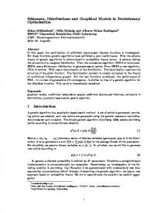
The interpretation of the parameter λ is clear: as in any signal detection problem, it is obviously difficult to detect an interaction θst if it is extremely close to zero. In contrast to classical signal detection problems, estimation of the graphical structure turns out to be harder if the edge parameters θst are large, since the large value of edge parameters can mask the presence of interactions on other edges. The following example illustrates this point: Example 1. Consider the family Gp,k of graphs on p = 3 with k = 2 edges; note that there are a total of 3 such graphs. For each of these three graphs, consider the parameter vector   θ(G) = θ θ 0 ,

where the single zero corresponds to the single distinct pair s 6= t not in the graph’s edge set, as illustrated in Figure 1. In the limiting case θ = +∞, for any choice of graph with two edges,

θ

θ

θ

θ θ

(a)

θ (b)

(c)

Figure 1. Illustration of the family Gp,k for p = 3 and k = 2; note that there are three distinct graphs G with p = 3 vertices and k = 2 edges. Setting the edge parameter θ(G) = [θ θ 0] induces a family of three Markov random fields. As the edge weight parameter θ increases, the associated distributions Pθ(G) become arbitrarily difficult to separate.

the Ising model distribution enforces the “hard-core” constraint that (X1 , X2 , X3 ) must  all be equal; that is, for any graph G, the distribution Pθ(G) places mass 1/2 on the configuration +1 +1 +1   and mass 1/2 on the configuration −1 −1 −1 . Of course, this hard-core limit is an extreme case, in which the models are not actually identifiable. Nonetheless, it shows that if the edge weight θ is finite but very large, the models will not identical, but nonetheless will be extremely hard to distinguish. Motivated by this example, we define the maximum neighborhood weight X ω ∗ (θ(G)) : = max |θst |. s∈V

4

t∈N (s)

(5)

Our analysis shows that the number of samples n required to distinguish graphs grows exponentially in this quantity. In this paper, we study classes of Markov random fields that are parameterized by a lower bound λ on the minimum edge weight, and an upper bound ω on the maximum neighborhood weight. Definition 1 (Classes of graphical models). (a) Given a pair (λ, ω) of positive numbers, the set Gp,d(λ, ω) consists of all distributions Pθ(G) of the form (2) such that (i) the underlying graph G = (V, E) is a member of the family Gp,d of graphs on p vertices with vertex degree at most d; (ii) the parameter vector θ = θ(G) respects the structure of G, meaning that θst 6= 0 only when (s, t) ∈ E, and (iii) the minimum edge weight and maximum neighborhood satisfy the bounds λ∗ (θ(G)) ≥ λ, and ω ∗ (θ(G)) ≤ ω. (6) (b) The set Gp,k (λ, ω) is defined in an analogous manner, with the graph G belonging to the class Gp,k of graphs with p vertices and k edges. We note that for any parameter vector θ(G), we always have the inequality ω ∗ (θ(G)) ≥ max |N (s)| λ∗ (θ(G)), s∈V

(7)

so that the families Gp,k (λ, ω) and Gp,d (λ, ω) are only well-defined for suitable pairs (λ, ω).

2.3

Graph decoders and error criterion

For a given graph class G (either Gp,d or Gp,k ) and positive weights (λ, ω), suppose that nature chooses some member Pθ(G) from the associated family G(λ, ω) of Markov random fields. Assume that the statistician observes n samples Xn1 : = {X (1) , . . . , X (n) } drawn in an independent and identically distributed (i.i.d.) manner from the distribution Pθ(G) . Note that by definition of the Markov random field, each sample X (i) belongs to the discrete set X : = {−1, +1}p , so that the overall data set Xn1 belongs to the Cartesian product space X n . We assume that the goal of the statistician is to use the data Xn1 to infer the underlying graph G ∈ G, which we refer to as the problem of graphical model selection. More precisely, we consider functions φ : X n → G, which we refer to as graph decoders. We measure the quality of a given graph decoder φ using the 0-1 loss function I[φ(Xn1 ) 6= G], which takes value 1 when φ(Xn1 ) 6= G and takes the value 0 otherwise, and we define associated 0-1 risk   Pθ(G) [φ(Xn1 ) 6= G] = Eθ(G) I[φ(Xn1 ) 6= G] ,

corresponding to the probability of incorrect graph selection. Here the probability (and expectation) are taken with the respect the product distribution of Pθ(G) over the n i.i.d. samples. The main purpose of this paper is to study the scaling of the sample sizes n—-more specifically, as a function of the graph size p, number of edges k, maximum degree d, minimum edge weight λ and maximum neighborhood weight ω—that are either sufficient for some graph decoder φ to output the correct graph with high probability, or conversely, are necessary for any graph decoder to output the correct graph with probability larger than 1/2. We study two variants of the graph selection problem, depending on whether the values of the edge weights θ are known or unknown. In the known edge weight variant, the task of the decoder is to distinguish between graphs, where for any candidate graph G = (V, E), the decoder knows the numerical values of the parameters θ(G). (Recall that by definition, [θ(G)]uv = 0 for all (u, v) ∈ / E, 5

so that the additional information being provided are the values [θ(G)]st for all (s, t) ∈ E.) In the unknown edge weight variant, both the graph structure and the numerical values of the edge weights are unknown. Clearly, the unknown edge variant is more difficult than the known edge variant. We prove necessary conditions (lower bounds on sample size) for the known edge variant, which are then also valid for the unknown variant. In terms of sufficiency, we provide separate sets of conditions for the known and unknown variants.

3

Main results and some consequences

In this section, we state our main results and then discuss some of their consequences. We begin with statement and discussion of necessary conditions in Section 3.1, followed by sufficient conditions in Section 3.2.

3.1

Necessary conditions

We begin with stating some necessary conditions on the sample size n that any decoder must satisfy for recovery over the families Gp,d and Gp,k . Recall (6) for the definitions of λ and ω used in the theorems to follow. Theorem 1 (Necessary conditions for Gp,d ). Consider the family Gp,d (λ, ω) of Markov random fields for some ω ≥ 1. If the sample size is upper bounded as n ≤ max



 exp(ω/4)dλ log( pd p d log p 4 − 1) , log , , , 2λ tanh(λ) 8 8d 128 exp( 3λ ) 2

(8)

then for any graph decoder φ : Xn1 → Gp,d , whether given known edge weights or not, max

θ(G)∈Gp,d (λ,ω)

  Pθ(G) φ(Xn1 ) 6= G ≥

1 . 2

(9)

Remarks: Let us make some comments regarding the interpretation and consequences of Theorem 1. First, suppose that both the maximum degree d and the minimum edge weight λ remain bounded (i.e., do not increase with the problem sequences). In this case, the necessary conditions (8) can be summarized more compactly as requiring that for some constant c, a sample size c log p n > λ tanh(λ) is required for bounded degree graphs. The observation of log p scaling has also been made in independent work [6], although the dependence on the signal-to-noise ratio λ given here is more refined. Indeed, note that if the minimum edge weight decreases to zero as the sample size ′ p is increases, then since λ tanh(λ) = O(λ2 ) for λ → 0, we conclude that a sample size n > c λlog 2 required, for some constant c′ . Some interesting phenomena arise in the case of growing maximum degree d. Observe that in the family Gp,d, we necessarily have ω ≥ λd. Therefore, in the case of growing maximum degree d → +∞, if we wish the bound (8) not to grow exponentially in d, it is necessary to impose the constraint λ = O( d1 ). But as observed previously, since λ tanh(λ) = O(λ2 ) as λ → 0, we obtain the following corollary of Theorem 1: Corollary 1. For the family Gp,d(λ, ω) with increasing maximum degree d, there is a constant c > 0 such that in a worst case sense, any method requires at least n > c max{d2 , λ−2 } log p samples to recover the correct graph with probability at least 1/2.

6

We note that Ravikumar et al. [22] have shown that under certain incoherence assumptions (roughly speaking, control on the Fisher information matrix of the distributions Pθ(G) ) and assuming that λ = Ω(d−1 ), a computationally tractable method using ℓ1 -regularization can recover graphs over the family Gp,d using n > c′ d3 log p samples, for some constant c′ ; consequently, Corollary 1 shows concretely that this scaling is within a factor d of information-theoretic bound. We now turn to some analogous necessary conditions over the family Gp,k of graphs on p vertices with at most k edges. Theorem 2 (Necessary conditions for Gp,k ). Consider the family Gp,k (λ, ω) of Markov random fields for some ω ≥ 1. If the sample size is upper bounded as   exp( ω2 ) log(k/8) log p , , , (10) n ≤ max 2λ tanh(λ) 64ω exp( 5λ 2 ) sinh(λ) then for any graph decoder φ : Xn1 → Gp,k , whether given known edge weights or not, max

θ(G)∈Gp,k (λ,ω)

  Pθ(G) φ(Xn1 ) 6= G ≥

1 . 2

(11)

Remarks: Again, we make some comments about the consequences of Theorem 2. First, suppose that both the number of edges k and the minimum edge weight λ remain bounded (i.e., do not increase with the problem sequences). In this case, the necessary conditions (10) can be summarized c log p more compactly as requiring that for some constant c, a sample size n > λ tanh(λ) is required for graphs with a constant number of edges. Again, note that if the minimum edge weight decreases to zero as the sample size increases, then since λ tanh(λ) = O(λ2 ) for λ → 0, we conclude that a ′ p is required, for some constant c′ . sample size n > c λlog 2 The behavior is more subtle in the case of graph sequences in which the number of edges k increases with the sample size. As shown in the proof of Theorem 2, it is √possible to construct a parameter vector θ(G) over a graph G with k edges such that ω ∗ (θ(G)) ≥ λ⌊ √k⌋. (More specifically, the construction is based on forming a completely connected subgraph on ⌊ k⌋ vertices, which has √
⌊ k⌋ ≤ k edges.) Therefore, if we wish to avoid the exponential growth from the a total of 2 term exp(ω), we require that λ = O(k−1/2 ) as the graph size increases. Therefore, we obtain the following corollary of Theorem 2: Corollary 2. For the family Gp,k (λ, ω) with increasing number of edges k, there is a constant c > 0 such that in a worst case sense, any method requires at least n > c max{k, λ−2 } log p samples to recover the correct graph with probability at least 1/2. To clarify a subtle point about comparing Theorems 1 and 2, consider a graph G ∈ Gp,d, say one with homogeneous degree d at each node. Note that such a graph has a total of k = dp/2 edges. Consequently, one might be misled into thinking Corollary 2 implies that n > c pd 2 log p samples would be required in this case. However, as shown in our development of sufficient conditions for the class Gp,d (see Theorem 3), this is not true for sufficiently small degrees d. To understand the difference, it should be remembered that our necessary conditions are worstcase results, based on adversarial choices from the graph families. As mentioned, the necessary conditions of Theorem 2 and hence of Corollary 2 are obtained by√ constructing a graph G that contains a completely connected graph, K√k , with uniform degree k. But K√k is not a member √ √ of Gp,d unless d ≥ k. On the other hand, for the case when d ≥ k, the necessary conditions of Corollary 1 amount to n > ck log p samples being required, which matches the scaling given in Corollary 2. 7

3.2

Sufficient conditions

We now turn to stating and discussing sufficient conditions (lower bounds on the sample size) for graph recovery over the families Gp,d and Gp,k . These conditions provide complementary insight to the necessary conditions discussed so far. Theorem 3 (Sufficient conditions for Gp,d ). (a) Suppose that for some n satisfies   3 3 exp(2ω) + 1  d 3 log p + log(2d) + log n ≥ sinh2 ( λ2 )

δ ∈ (0, 1), the sample size 1 . δ

(12)

Then there exists a graph decoder φ∗ : Xn1 → Gp,d such that given known edge weights, the worst-case error probability satisfies  max Pθ(G) φ∗ (Xn1 ) 6= G] ≤ δ. (13) θ(G)∈Gp,d (λ,ω)

(b) In the case of unknown edge weights, suppose that the sample size satisfies h ω 3 exp(2ω + 1
i2  16 log p + 4 log(2/δ) . n > 2 sinh (λ/4)

(14)

Then there exists a graph decoder φ† : Xn1 → Gp,d that that has worst-case error probability at most δ. Remarks: It is worthwhile comparing the sufficient conditions provided by Theorem 3 to the necessary conditions from Theorem 1. First, consider the case of finite degree graphs. In this case, the condition (12) reduces to the statement that for some constant c, it suffices to have n > c λ−2 log p samples. Comparing with the necessary conditions (see the discussion following Theorem 1), we see that for known edge weights and bounded degrees, the information-theoretic capacity scales as λ−2 log p. For unknown edge weights, the conditions (14) provide a weaker guarantee, namely that n > c′ λ−4 log p samples are required; we suspect that this guarantee could be improved by a more careful analysis. In the case of growing maximum graph degree d, we note that like the necessary conditions (8), the sample size specified by the sufficient conditions (12) scales exponentially in the parameter ω. If we wish not to incur such exponential growth, we necessarily must have that λ = O(1/d). We thus obtain the following consequence of Theorem 3: Corollary 3. For the graph family Gp,d(λ, ω) with increasing maximum degree, there exists a graph decoder that succeeds with high probability using n > c1 max{d2 , λ−2 d log p samples.

This corollary follows because the scaling λ = O(1/d) implies that λ → 0 as d increases, and sinh(λ/2) = O(λ) as λ → 0. Note that in this regime, Corollary 1 of Theorem 1 showed that no method has error probability below 1/2 if n < c2 max{d2 , λ−2 } log p, for some constant c2 . Therefore, together Theorems 1 and 3 provide upper and lower bounds on the sample complexity of graph selection that are matching to within a factor of d. We note that under the condition λ ≥ cd3 , the results of Ravikumar et al. [22] also guarantee correct recovery with high probability for n > c4 d3 log p using ℓ1 -regularized logistic regression; however, their method requires additional (somewhat restrictive) incoherence assumptions that are not imposed here. Finally, we state sufficient conditions for the class Gp,k in the case of known edge weights: 8

Theorem 4 (Sufficient conditions for Gp,k ). (a) Suppose that for some δ ∈ (0, 1), the sample size n satisfies n >

3 exp(2ω) + 1 1
(k + 1) log p + log . 2 λ δ sinh ( 4 )

Then for known edge weights, there exists a graph decoder φ∗ : Xn1 → Gp,k such that  max Pθ(G) φ∗ (Xn1 ) 6= G] ≤ δ. θ(G)∈Gp,k (λ,ω)

(15)

(16)

(b) For unknown edge weights, there also exists a graph decoder that succeeds under the condition (14). Remarks: It is again interesting to compare Theorem 4 with the necessary conditions from Theorem 2. To begin, let the number of edges k remain bounded. In this case, for λ = o(1), condition (15) p samples, which matches (up to constant states that for some constant c, it suffices to have n > c log λ2 factors) the lower bound implied by Theorem 2. In the more general setting of k → +∞, we begin by noting that like in Theorem 2, the sample size in Theorem 4 grows exponentially unless the parameter ω stays controlled. As with the discussion following Theorem 2, one interesting scaling is to require that λ ≍ k−1/2 , a choice which controls the worst-case construction that leads to the factor exp(ω) in the proof of Theorem 2. With this scaling, we have the following consequence: Corollary 4. Suppose that the minimum value λ scales with the number of edges k as λ ≍ k−1/2 . Then in the case of known edge weights, there exists a decoder that succeeds with high probability using n > ck2 log p samples. Note that these sufficient conditions are within a factor of k of the necessary conditions from Corollary 2, which show that unless n > c′ max{k, λ−2 } log p, then any graph estimator fails at least half of the time.

4

Proofs of necessary conditions

In the following two sections, we provide the proofs of our main theorems. We begin by introducing some background on distances between distributions, as well as some results on the cardinalities of our model classes. We then provide proofs of the necessary conditions (Theorems 1 and 2) in this section, followed by the proofs of the sufficient conditions stated in Theorems 3 and 4 in Section 5.

4.1

Preliminaries

We begin with some preliminary definitions and results concerning “distance” measures between different models, and some estimates of the cardinalities of different model classes. 4.1.1

Distance measures

In order to quantify the distinguishability of different models, we begin by defining some useful p “distance” measures. Given two parameters θ and θ ′ in R(2) , we let D(θ k θ ′ ) denote the KullbackLeibler divergence [10] between the two distributions Pθ and Pθ′ . For the special case of the Ising model distributions (2), this Kullback-Leibler divergence takes the form D(θ k θ ′ ) : =

X

x∈{−1,+1}p

9

Pθ (x) log

Pθ (x) . Pθ′ (x)

(17)

Note that the Kullback-Leibler divergence is not symmetric in its arguments (i.e., D(θ k θ ′ ) 6= D(θ k θ ′ ) in general). Our analysis also makes use of two other closely related divergence measures, both of which are symmetric. First, we define the symmetrized Kullback-Leibler divergence, defined in the natural way via S(θ k θ ′ ) : = D(θ k θ ′ ) + D(θ ′ k θ).

(18)

Secondly, given two parameter vectors θ and θ ′ , we may consider the model P θ+θ′ specified by their 2 average. In terms of this averaged model, we define another type of divergence via θ + θ′ θ + θ′ ′ k θ) + D( k θ ). (19) 2 2 Note that this divergence is also symmetric in its arguments. A straightforward calculation shows that this divergence measure can be expressed in terms of the cumulant function (3) associated with the Ising family as J(θ k θ ′ ) : = D(

J(θ k θ ′ ) = log

Z(θ)Z(θ ′) . ′ Z 2 ( θ+θ ) 2

(20)

Useful in our analysis are representations of these distance measures in terms of the vector of p mean parameters µ(θ) ∈ R(2) , where element µst is given by X µst : = Eθ [Xs Xt ] = Pθ [X] Xs Xt . (21) x∈{−1,+1}p

It is well-known from the theory of exponential families [7, 28] that there is a bijection between the canonical parameters θ and the mean parameters µ. Using this notation, a straightforward calculation shows that the symmetrized Kullback-Leibler divergence between Pθ and Pθ′ is equal to X

′ S(θ k θ ′ ) = θst − θst µst − µ′st , (22) s,t∈V,s6=t

where µst and µ′st denote the edge-based mean parameters under θ and θ ′ respectively. 4.1.2

Cardinalities of graph classes

In addition to these divergence measures, we require some estimates of the cardinalities of the graph classes Gp,d and Gp,k , as summarized in the following:
Lemma 1. (a) For k ≤ p2 /2, the cardinality of Gp,k is bounded as  p
  p
 2 (23) ≤ |Gp,k | ≤ k 2 , k k and hence log Gp,k = Θ(k log √pk ). (b) For d ≤

p−1 2 ,

the cardinality of Gp,d is bounded as

 d(d+1)  p
  2 pd 2 p ≤ |Gp,d | ≤ ⌋! ⌊ pd . d+1 2 2 p
and hence log Gp,d = Θ pd log d . 10

(24)

p
Proof. (a) For the bounds (23) on |Gp,k |, we observe that there are (2ℓ) graphs with exactly ℓ p
p

edges, and that for k ≤ p2 /2, we have (2ℓ) ≤ (k2) for all ℓ = 1, 2, . . . , k. (b) Turning to the bounds (24) on |Gp,d |, observe that every model in Gp,d has at most pd 2 edges. p−1 Note that d ≤ 2 ensures that   pd p ≤ /2. 2 2 p
pd Therefore, following the argument in part (a), we conclude that |Gp,d | ≤ pd 2 2 2 as claimed. In order to establish the lower bound (24), we first group the p vertices into d + 1 groups of p size ⌊ d+1 ⌋, discarding any remaining vertices. We consider a subset of Gp,d : graphs with maximum degree d having the property that each component edge straddles vertices in two different groups. p ⌋, and form an bijection from group To construct one such graph, we pick a permutation of ⌊ d+1 1 to group 2 corresponding to the permutation. Similarly, we form an bijection from group 1 to 3, and so on up until d + 1. Note that use d permutations to complete this procedure, and at the end of this round, every vertex in group 1 has degree d, vertices in all other groups have degree 1. Similarly, in the next round, we use d − 1 permutations to connect group 2 to groups 3 through d + 1. In general, for i = 1, . . . , d, in round i, we use d + 1 − i permutations to connect group i with groups i + 1, . . . , d + 1. Each choice of these permutations yields a distinct graph in Gp,d. Note that we use a total of

d d X X d (d + 1) (d + 1 − i) = ℓ = 2 i=1

permutations over 4.1.3

p ⌊ d+1 ⌋

ℓ=1

elements, from which the stated claim (24) follows.

Fano’s lemma and variants

We provide some background on Fano’s lemma and its variants needed in our arguments. Consider a family of M models indexed by the parameter vectors {θ (1) , θ (2) , . . . , θ (M ) }. Suppose that we choose a model index k uniformly at random from {1, . . . , M }, and than sample a data set Xn1 of n samples drawn in an i.i.d. manner according to a distribution Pθ(k) . In this setting, Fano’s lemma provides a lower bound on the probability of error of any classification function φ : X n → {1, . . . , M }, specified in terms of the mutual information I(Xn1 ; K) = H(Xn1 ) − H(Xn1 | K)

(25)

between the data Xn1 and the random model index K. We say that a decoder φ : X n → {1, . . . , M } is unreliable over the family {θ (1) , . . . , θ (M ) } if  max Pθ(k) φ(Xn1 ) 6= k] ≥

k=1,...,M

1 . 2

(26)

We summarize Fano’s inequality and a variant thereof in the following lemma: Lemma 2. Any of the following upper bounds on the sample size imply that any decoder φ is unreliable over the family {θ (1) , . . . , θ (M ) }: (a) The sample size n is upper bounded as n
3m/4 and j < m/4. Accordingly, we may choose a maximizing point j ∗ > 3m/4. Since all the terms in the numerator are non-negative, we have  ∗ 
m
λ 2 Pθ(Gst ) [Xs Xt = +1] j ∗ exp 2 (2j − m + 1) − 4  

≥ Pθ(Gst ) [Xs Xt = −1] (m + 1) jm∗ exp λ2 (2j ∗ − m)2  
exp λ2 4j ∗ − 2m − 3 = m+1  
exp λ2 m − 3 ≥ m+1
exp ω2 − 23 λ = , m+1 which completes the proof of the bound (29).

4.3

Proof of Theorem 1

We begin with necessary conditions for the bounded degree family Gp,d . The proof is based on applying Fano’s inequality to three ensembles of graphical models, each contained within the family Gp,d (λ, ω).
Ensemble A: In this ensemble, we consider the set of p2 graphs, each of which contains a single edge. For each such graph—say the one containing edge (s, t), which we denote by Hst—we set [θ(Hst )]st = λ, and all other entries equal to zero. Clearly, the resulting Markov random fields Pθ(H) all belong to the family Gp,d(λ, ω). (Note that by definition, we must have ω ≥ λ for the family to be non-empty.) Let us compute the symmetrized Kullback-Leibler divergence between the MRFs indexed by θ(Gst ) and θ(Guv ). Using the representation (22), we have  

S(θ(Hst) k θ(Huv )) = λ Eθ(Hst ) [Xs Xt ] − Eθ(Huv ) [Xs Xt ] − Eθ(Hst ) [Xu Xv ] − Eθ(Huv ) [Xu Xv ] = 2λEθ(Hst ) [Xs Xt ],

since Eθ(Hst ) [Xu Xv ] = 0 for all (u, v) 6= (s, t), and Eθ(Huv ) [Xu Xv ] = Eθ(Hst ) [Xs Xt ]. Finally, by definition of the distribution Pθ(Hst ) , we have Eθ(Hst ) [Xs Xt ] =

exp(λ) − exp(−λ) = tanh(λ), exp(λ) + exp(−λ)

so that we conclude that the symmetrized Kullback-Leibler divergence is equal to 2λ tanh(λ) for each pair. 13


Using the bound (28) from Lemma 2 with M = p2 , we conclude that the graph recovery is unreliable (i.e., has error probability above 1/2) if the sample size is upper bounded as
log( p2 /4) . (32) n < λ tanh(λ) Ensemble B: In order to form this graph ensemble, we begin with a grouping of the p vertices into p ⌊ d+1 ⌋ groups, each with d + 1 vertices. We then consider the graph G obtained by fully connecting p ⌋ cliques of size d + 1. each subset of d + 1 vertices. More explicitly, G is a graph that contains ⌊ d+1 Using this base graph, we form a collection of graphs by beginning with G, and then removing a single edge (u, v). We denote the resulting graph by Guv . Note that if p ≥ 2(d + 1), then we can form   p d+1 pd ⌊ ⌋ ≥ d+1 2 4 such graphs. For each graph Guv , we form an associated Markov random field Pθ(Guv ) by setting [θ(Guv )]ab = λ > 0 for all (a, b) in the edge set of Guv , and setting the parameter to zero otherwise. A central component of the argument is the following bound on the symmetrized KullbackLeibler divergence between these distributions Lemma 2. For all distinct pairs of models θ(Gst ) 6= θ(Guv ) in ensemble B and for all λ ≥ 1/d, the symmetrized Kullback-Leibler divergence is upper bounded as S(θ(Gst ) k θ(Guv )) ≤

8λ d exp( 3λ 2 ) exp( λd 2 )

.

Proof. Note that any pair of distinct parameter vectors θ(Gst ) 6= θ(Guv ) differ in exactly two edges. Consequently, by the representation (22), and the definition of the parameter vectors,

S(θ(Gst ) k θ(Guv )) = λ Eθ(Guv ) [Xs Xt ] − Eθ(Gst ) [Xs Xt ] + λ Eθ(Gst ) [Xu Xv ] − Eθ(Guv ) [Xu Xv ]

≤ λ 1 − Eθ(Gst ) [Xs Xt ] + λ 1 − Eθ(Guv ) [Xu Xv ] ,

where the inequality uses the fact that λ > 0, and the edge-based mean parameters are upper bounded by 1. p ⌋ cliques, we Since the model Pθ(Gst ) factors as a product of separate distributions over the ⌊ d+1 can now apply the separation result (30) from Lemma 1 with m = d + 1 to conclude that S(θ(Gst ) k θ(Guv )) ≤ 2λ ≤

2 (d + 2) exp( 3λ 2 ) exp( λ(d+1) ) + (d + 2) exp( 3λ 2 2 )

8 λ d exp( 3λ 2 ) exp( λd 2 )

,

as claimed. Using Lemma 2 and applying the bound (28) from Lemma 2 with M = probability of error below 1/2 and λd ≥ 2, we require at least n >

pd exp( dλ log( pd 4 − 1) 2 ) log( 4 − 1) ≥ S(θ(Gst ) k θ(Guv )) 8dλ exp( 3λ 2 )

14

pd 4

yields that for

samples. Since exp(t/4) ≥ t2 /16 for all t ≥ 1, we certainly need at least n > samples. Since ω = dλ in this construction, we conclude that n >

exp(dλ/4)dλ log( pd −1) 4 128 exp( 3λ ) 2

exp(ω/4)dλ log( pd 4 − 1) 128 exp( 3λ 2 )

samples are required, as claimed in Theorem 1. Ensemble C: Finally, we prove the third component in the bound (8). In this case, we consider the ensemble consisting of all graphs in Gp,d . From Lemma 1(b), we have log |Gp,d | ≥ ≥ ≥

d(d + 1) p log ⌊ ⌋! 2 d+1 ⌊ p ⌋ d(d + 1) p ⌊ ⌋ log d+1 2 d+1 e p dp log . 4 8d

For this ensemble, it suffices to use a trivial upper bound on the mutual information (25), namely I(Xn1 ; G) ≤ H(Xn1 ) ≤ np, where the second bound follows since Xn1 is a collection of np binary variables, each with entropy at most 1. Therefore, from the Fano bound (27), we conclude that the error probability stays above p , as claimed. 1/2 if the sample size n is upper bounded as n < d8 log 8d

4.4

Proof of Theorem 2

We now turn to the proof of necessary conditions for the graph family Gp,k with at most k edges. As with the proof of Theorem 2, it is based on applying Fano’s inequality to three ensembles of Markov random fields contained in Gp,k (λ, ω). Ensemble A: Note that the ensemble (A) previously constructed in the proof of Theorem 1 is also valid for the family Gp,k (λ, ω), and hence the bound (32) is also valid for this family.
Ensemble B: For this ensemble, we choose the largest integer m such that k + 1 ≥ m 2 . Note that we certainly have √   √ m k . ≥ ⌊ k⌋ ≥ 2 2
We then form a family of m 2 graphs as follows: (a) first form the complete graph Km on a subset of m vertices, and (b) for each (s, t) ∈ Km , form the graph Gst by removing edge (s, t) from Km . We form Markov random fields on these graphs by setting [θ(Gst )]wz = λ if (w, z) ∈ E(Gst ), and setting it to zero otherwise. Lemma 3. For all distinct model pairs θ(Gst ) and θ(Guv ), we have S(θ(Gst ) k θ(Guv )) ≤

15

16ω exp( 5λ 2 ) sinh(λ) . exp( ω2 )

(33)

Proof. We begin by claiming for any pair (s, t) 6= (u, v), the distribution Pθ(Guv ) (i.e., corresponding to the subgraph that does not contain edge (u, v)) satisfies Pθ(Guv ) [Xs Xt = +1] Pθ(Guv ) [Xs Xt = −1]

≤ exp(2λ)

Pθ(Gst ) [Xs Xt = +1] qst = exp(2λ) , Pθ(Gst ) [Xs Xt = −1] 1 − qst

(34)

where we have re-introduced the convenient shorthand qst = Pθ(Gst ) [Xs Xt = 1] from Lemma 1. To prove this claim, let Pθ be the distribution that contains all edges in the complete subgraph Km , each with weight λ. Let Z(θ) and Z(θ(Guv )) be the normalization constants associated with Pθ and Pθ(Guv ) respectively. Now since λ > 0 by assumption, by the FKG inequality [2], we have Pθ(Guv ) [Xs Xt = +1] Pθ(Guv ) [Xs Xt = −1]

Pθ [Xs Xt = +1] Pθ [Xs Xt = −1]

≤

We now apply the definition of Pθ and expand the right-hand side of this expression, recalling the fact that the model Pθ(Gst ) does not contain the edge (s, t). Thus we obtain Pθ [Xs Xt = +1] Pθ [Xs Xt = −1]

st ))

=

exp(λ) Z(θ(G Z(θ)

Pθ(Gst ) [Xs Xt = +1]

st )) exp(−λ) Z(θ(G Z(θ)

Pθ(Gst ) [Xs Xt = −1]

Pθ(Gst ) [Xs Xt = +1] , Pθ(Gst ) [Xs Xt = −1]

= exp(2λ)

which establishes the claim (34). Finally, from the representation (22) for the symmetrized Kullback-Leibler divergence and the definition of the models,   S(θ(Gst ) k θ(Guv )) = λ Eθ(Gst ) [Xu Xv ] − Eθ(Guv ) [Xu Xv ] + λ Eθ(Guv ) [Xs Xt ] − Eθ(Gst ) [Xs Xt ]  = 2λ Eθ(Guv ) [Xs Xt ] − Eθ(Gst ) [Xs Xt ] ,

where we have used the symmetry of the two terms. Continuing on, we observe the decomposition Eθ(Gst ) [Xs Xt ] = 1 − 2Pθ(Gst ) [Xs Xt = −1], and using the analogous decomposition for the other expectation, we obtain  S(θ(Gst ) k θ(Guv )) = 4λ Pθ(Gst ) [Xs Xt = −1] − Pθ(Guv ) [Xs Xt = −1] n o 1 1 = 4λ P − Pθ(Guv ) [Xs Xt =+1] θ(Gst ) [Xs Xt =+1] +1 P uv [Xs Xt =−1] P [X X =−1] + 1 θ(Gst )

(a)

≤

= =

n 4λ

s

1 qst 1−qst

4λ n

qst 1−qst

+1

θ(G

t

−

1 qst exp(2λ) 1−q st

1 1+

1−qst qst

4λ (exp(2λ) − 1) qst 1−qst

)

− 

1 exp(2λ) + 1+

1−qst  qst

+1

o

1−qst qst



o

1 exp(2λ) +

1−qst  qst

where in obtaining the inequality (a), we have applied the bound (34) and recalled our shorthand notation qst = Pθ(Gst ) [Xs Xt = +1]. Since λ > 0 and (1−qst )/qst ≥ 0, both terms in the denominator

of the second term are at least one, so that we conclude that S(θ(Gst ) k θ(Guv )) ≤ 16

4λ (exp(2λ)−1) qst 1−qst

.

Finally, applying the lower bound (29) from Lemma 1 on the ratio qst /(1 − qst ), we obtain that S(θ(Gst ) k θ(Guv )) ≤ ≤

4λ (exp(2λ) − 1) (m + 1) exp( ω2 − 32 λ) 16ω exp( 5λ 2 ) sinh(λ) , exp( ω2 )

where we have used the fact that λ (m + 1) ≤ 2mλ = 2ω. By combining Lemma 3 with Lemma 2(b), we conclude that for correctness with probability at least 1/2, the sample size n must be at least n >

exp( ω2 ) log

(m2 ) 4

32ω exp( 5λ 2 ) sinh(λ)

≥

exp( ω2 ) log(k/8) 64ω exp( 5λ 2 ) sinh(λ)

,

as claimed in Theorem 2.

5

Proofs of sufficient conditions

We now turn to the proofs of the sufficient conditions given in Theorems 3 and 4, respectively, for the classes Gp,d and Gp,k . In both cases, our method involves a direct analysis of a maximum likelihood (ML) decoder, which searches exhaustively over all graphs in the given class, and computes the model with highest likelihood. We begin by describing this ML decoder and providing a standard large deviations bound that governs its performance. The remainder of the proof involves more delicate analysis to lower bound the error exponent in the large deviations bound in terms of the minimum edge weight λ and other structural properties of the distributions.

5.1

ML decoding and large deviations bound

Given a collection Xn1 = {X (1) , . . . , X (n) } of n i.i.d. samples, its (rescaled) likelihood with respect to model Pθ is given by n

ℓθ (Xn1 ) : =

1X log Pθ [X (i) ]. n

(35)

i=1

For a given graph class G and an associated set of graphical models {θ(G) | G ∈ G}, the maximum likelihood decoder is the mapping φ∗ : X → G defined by φ∗ (Xn1 ) = arg max ℓθ(G) (Xn1 ). G∈G

(36)

(If the maximum is not uniquely achieved, we choose some graph G from the set of models that attains the maximum.) Suppose that the data is drawn from model Pθ(G) for some G ∈ G. Then the ML decoder φ∗ fails only if there exists some other θ(G′ ) 6= θ(G) such that ℓθ(G′ ) (Xn1 ) ≥ ℓθ(G) (Xn1 ). (Note that we are being conservative by declaring failure when equality holds). Consequently, by union bound, we have X   Pθ [φ∗ (Xn1 ) 6= G] ≤ P ℓθ(G′ ) (Xn1 ) ≥ ℓθ(G) (Xn1 ) G′ ∈G\G

Therefore, in order to provide sufficient conditions for the error probability of the ML decoder to vanish, we need to provide an appropriate large deviations bound. 17

Lemma 3. Given n i.i.d. samples Xn1 = {X (1) , . . . , X (n) } from Pθ(G) , for any G′ 6= G, we have   n P ℓθ(G′ ) (Xn1 ) ≥ ℓθ(G) (Xn1 ) ≤ exp − J(θ(G) k θ(G′ )), 2

(37)

where the distance S was defined previously (19). Proof. So as to lighten notation, let us write θ = θ(G) and θ ′ = θ(G′ ). We apply the Chernoff bound to the random variable V = ℓθ′ (Xn1 ) − ℓθ (Xn1 ), thereby obtaining that   1 inf log Eθ exp(sV ) n s>0 X s  1−s  Pθ (x) Pθ′ (x) = inf

1 log Pθ [V ≥ 0] ≤ n

s>0

x∈{−1,+1}p

≤ log Z θ/2 + θ ′ /2) −

1 1 log Z(θ) − log Z(θ ′ ), 2 2

where Z(θ) denotes the normalization constant associated with the Markov random field Pθ , as defined in equation (3). The claim then follows by applying the representation (20) of J(θ k θ ′ ).

5.2

Lower bounds based on matching

In order to exploit the large deviations claim in Lemma 3, we need to derive lower bounds on the divergence J(θ(G) k θ(G′ )) between different models. Intuitively, it is clear that this divergence is related to the discrepancy of the edge sets of the two graph. The following lemma makes this intuition precise. We first recall some standard graph-theoretic terminology: a matching of a graph G = (V, E) is a subgraph H such that each vertex in H has degree one. The matching number of G is the maximum number of edges in any matching of G. Lemma 4. Given two distinct graphs G = (V, E) and G′ = (V, E ′ ), let m(G, G′ ) be the matching number of the graph with edge set E∆E ′ : = (E\E ′ ) ∪ (E ′ \E ′ ). Then for any pair of parameter vectors θ(G) and θ(G′ ) in G(λ, ω), we have J(θ(G) k θ(G′ )) ≥

m(G, G′ ) λ sinh2 ( ). 3 exp(2ω) + 1 4

(38)

Proof. Some comments on notation before proceeding: we again adopt the shorthand notation θ = θ(G) and θ ′ = θ(G′ ). In this proof, we use ej to denote either a particular edge, or the set of two vertices that specify the edge, depending on the context. Given any subset A ⊂ V , we use xA = {xs , s ∈ A} to denote the collection of variables indexed by A. Given any edge e = (u, v) with u ∈ / A and v ∈ / A, we define the conditional distribution Peθ[xA ] (xu , xv ) =

Pθ (xu , xv , xA ) Pθ (xA )

(39)

over the random variables xe = (xu , xv ) indexed by the edge. Finally, we use

JxeA (θ k θ ′ ) : = D Peθ[xA ]+θ′ [xA ] k Peθ[xA ] + D Peθ[xA ]+θ′ [xA ] k Peθ′ [xA ] 2

2

18

(40)

to denote the divergence (19) applied to the conditional distributions of (Xu , Xv | XA = xA ). With this notation, let M ⊂ E∆E ′ be the subset of edges in some maximal matching of the graph with edge set E∆E ′ ; concretely, let us write M = {e1 , . . . , em }, and denote by V \M the subset of vertices that are not involved in the matching. Note that since J is a combination of Kullback-Leibler (KL) divergences, the usual chain rule for KL divergences [10] also applies to it. Consequently, we have ′

J(θ k θ ) ≥

m X

X

xV \M ,xe1 ,...xeℓ−1

ℓ=1

P θ+θ′ (xV \M , xe1 , . . . , xeℓ−1 ) JxeSℓ 2

ℓ−1

(θ k θ ′ ),


where for each ℓ, we are conditioning on the set of variables xSℓ−1 : = xV \M , xe1 , . . . , xeℓ−1 . Finally, from Lemma 7 in Appendix A, for all ℓ = 1, . . . , m and all values of xSℓ−1 , we have JxeSℓ

ℓ−1

(θ k θ ′ ) ≥

λ 1 sinh2 ( ), 3 exp(2ω) + 1 4

from which the claim follows.

5.3

Proof of Theorem 3(a)

We first consider distributions belonging to the class Gp,d (λ, ω), where λ is the minimum absolute value of any non-zero edge weight, and ω is the maximum neighborhood weight (5). Consider a pair of graphs G and G′ in the class Gp,d that differ in ℓ = |E ∆E ′ | edges. Since both graphs have maximum degree at most d, we necessarily have a matching number m(G, G′ ) ≥ 4ℓd . Note that the parameter ℓ = |E ∆E ′ | can range from 1 all the way up to dp, since a graph with maximum degree d has at most dp 2 edges. Now consider some fixed graph G ∈ Gp,d and associated distribution Pθ(G) ∈ Gp,d; we upper p
bound the error probability P [φ∗ (Xn ) 6= G]. For each ℓ = 1, 2, . . . , dp, there are at most (2) θ(G)

1

ℓ

models in Gp,d with mismatch ℓ from G. Therefore, applying the union bound, the large deviations bound in Lemma 3, and the lower bound in terms of matching from Lemma 4, we obtain ∗

Pθ(G) [φ

(Xn1 )

pd  X

p
 2

λ o ℓ/(4d) sinh2 ( ) 3 exp(2ω) + 1 2 ℓ ℓ=1
  p n ℓ/(4d) λ o ≤ pd max exp log 2 − n sinh2 ( ) ℓ=1,...,pd ℓ 3 exp(2ω) + 1 2 n λ o ℓ/(4d) sinh2 ( ) . ≤ max exp log(pd) + ℓ log p − n ℓ=1,...,pd 3 exp(2ω) + 1 2

6= G] ≤

exp

n

−n

This probability is at most δ under the given conditions on n in the statement of Theorem 3(a).

5.4

Proof of Theorem 4

Next we consider the class Gp,k of graphs with at most k edges. Given some fixed graph G ∈ Gp,k , consider some other graph G′ ∈ Gp,k such that the set E ∆ E ′ has cardinality m. We claim that for each m = 1, 2, . . . , 2k, the number of such graphs is at most To verify this claim, recall the notion of a vertex cover of a set of edges, namely a subset of vertices such that each edge in the set is incident to at least one vertex of the set. Note also that the 19

vertices involved in any maximal matching form a vertex cover. Consequently, any maximal matching over the edge set E ∆ E ′ of cardinality m be described in the following (suboptimal) fashion: (i) first specify which of the k edges in E are missing in E ′ ; (ii) describe which of the at most 2m vertices belong to the vertex cover defined by the maximal matching; and (iii) describe the subset of at most k vertices that are connected to it. This procedure yields at most 2k p2m p2 k m = 2k p2m (k+1) possibilities, as claimed. Consequently, applying the union bound, the large deviations bound in Lemma 3, and the lower bound in terms of matching from Lemma 4, we obtain Pθ(G) [φ∗ (Xn1 ) 6= G] ≤

k X

2k p2 m (k+1) exp

m=1

≤ k max

m=1,...,k

n

−n

m λ o sinh2 ( ) 3 exp(2ω) + 1 2

n exp k + 2m(k + 1) log p − n

λ o m sinh2 ( ) . 3 exp(2ω) + 1 2

This probability is less than δ under the conditions of Theorem 4, which completes the proof.

5.5

Proof of Theorems 3(b) and 4(b)

Finally, we prove the sufficient conditions given in Theorem 3(b) and 4(b), which do not assume that the decoder knows the parameter vector θ(G) for each graph G ∈ Gp,d. In this case, the simple ML decoder (36) cannot be applied, since it assumes knowledge of the model parameters θ(G) for each graph G ∈ Gp,d . A natural alternative would be the generalized likelihood ratio approach, which would maximize the likelihood over each model class, and then compare the maximized likelihoods. Our proof of Theorem 3(b) is based on minimizing the distance between the empirical and model mean parameters in the ℓ∞ norm, which is easier to analyze. 5.5.1

Decoding from mean parameters

We begin by describing the graph decoder used to establish the sufficient conditions of Theop p rem 3(b). For any parameter vector θ ∈ R(2) , let µ(θ) ∈ R(2) represent the associated set of mean parameters, with element (s, t) given by [µ(θ)]st : = Eθ [Xs Xt ]. Given a data set Xn1 = {X (1) , . . . , X (n) }, the empirical mean parameters are given by n

µ bst : =

1 X (i) (i) Xs Xt . n

(41)

i=1

p

For a given graph G = (V, E), let Θλ,ω (G) ⊂ R(2) be a subset of exponential parameters that respect the graph structure—viz. (a) we have θuv = 0 for all (u, v) ∈ / E; (b) for all edges (s, t) ∈ E, we have |θst | ≥ λ, and P (c) for all vertices s ∈ V , we have t∈N (s) |θst | ≤ ω.

p For any graph G and set of mean parameters µ ∈ R(2) , we define a projection-type distance via JG (µ) = minθ∈Θλ,ω (G) kµ − µ(θ)k∞ . We now have the necessary ingredients to define a graph decoder φ† : X n → Gp,d; in particular, it is given by

µ), φ† (Xn1 ) : = arg min JG (b G∈Gp,d

20

(42)

where µ b are the empirical mean parameters previously defined (41). (If the minimum (42) is not uniquely achieved, then we choose some graph that achieves the minimum.) 5.5.2

Analysis of decoder

Suppose that the data are sampled from Pθ(G) for some fixed but known graph G ∈ Gp,d , and parameter vector θ(G) ∈ Θλ,ω (G). Note that the graph decoder φ† can fail only if there exists some µ) − JG (b µ) is not positive. (Again, we other graph G′ such that the difference ∆(G′ ; G) : = JG′ (b are conservative in declaring failure if there are ties.) µ), so that Let θ ′ denote some element of Θλ,ω (G′ ) that achieves the minimum defining JG′ (b ′ b µ) = kb µ − µ(θ )k∞ . Note that by the definition of JG , we have JG (G) ≤ kb µ − θ(G)k∞ , where JG′ (b θ(G) are the parameters of the true model. Therefore, by the definition of ∆(G′ ; G), we have ∆(G′ ; G) ≥ kb µ − µ(θ ′ )k∞ − kb µ − µ(θ(G))k∞

≥ kµ(θ ′ ) − µ(θ(G))k∞ − 2kb µ − µ(θ(G))k∞ ,

(43)

where the second inequality applies the triangle inequality. Therefore, in order to prove that ∆(G′ ; G) is positive, it suffices to obtain an upper bound on kb µ − µ(θ(G))k∞ , and a lower bound on kµ(θ ′ ) − µ(θ(G))k∞ , where θ ′ ranges over Θλ,ω (G′ ). With this perspective, let us state two key lemmas. We begin with the deviation between the sample and population mean parameters: Lemma 5 (Elementwise deviation). Given n i.i.d. samples drawn from Pθ(G) , the sample mean parameters µ b and population mean parameters µ(θ(G)) satisfy the tail bound P[kb µ − µ(θ(G))k∞ ≥ t] ≤ 2 exp − n

This probability is less than δ for t ≥

q


t2 + 2 log p . 2

4 log p+log(2/δ) . n

Our second lemma concerns the separation of the mean parameters of models with different graph structure: Lemma 6 (Pairwise separations). Consider any two graphs G = (V, E) and G′ = (V, E ′ ), and an associated set of model parameters θ(G) ∈ Θλ,ω (G) and θ(G′ ) ∈ Θλ,ω (G′ ). Then for all edges (s, t) ∈ E\E ′ ∪ E ′ \E, max

u∈{s,t},v∈V

Eθ(G) [Xu Xv ] − Eθ(G′ ) [Xu Xv ] ≥

sinh2 (λ/4)
. 2ω 3 exp(2ω) + 1

We provide the proofs of these two lemmas in Sections 5.5.3 and 5.5.4 below. Given these two lemmas, we can complete the proofs of Theorem 3(b) and Theorem 4(b). Using the lower bound (43), with probability greater than 1 − δ, we have r sinh2 (λ/4) 4 log p + log(2/δ) ′
−2 ∆(G ; G) ≥ . n ω 3 exp(2ω + 1

This quantity is positive as long as h ω 3 exp(2ω + 1
i2  16 log p + 4 log(2/δ) , n > 2 sinh (λ/4) which completes the proof. It remains to prove the auxiliary lemmas used in the proof. 21

5.5.3

Proof of Lemma 5

This claim is an elementary consequence of the Hoeffding bound. By definition, for each pair (s, t) of distinct vertices, we have n

µ bst − [µ(θ(G))]st =

1 X (i) (i) Xs Xt − Eθ(G) [Xs Xt ], n i=1

(i)

(i)

which is the deviation of a sample mean from its expectation. Since the random variables {Xs Xt }ni=1 are i.i.d. and lie in the interval [−1, +1], an application of Hoeffding’s inequality [16] yields that P[ µ bst − [µ(θ(G))]st ≥ t] ≤ 2 exp − nt2 /2). p
The lemma follows by applying union bound over all 2 edges of the graph, and the fact that
p log 2 ≤ 2 log p. 5.5.4

Proof of Lemma 6

The proof of this claim is more involved. Let (s, t) be an edge in E\E ′ , and let C be the set of all other vertices that are adjacent to s or t in either graphs—namely, the set 
C : = u ∈ V | (u, s) or (u, t) ∈ E ∪ E ′ = N (s) ∪ N (t) \{s, t}.

Our approach is to condition on the variables xC = {xu , u ∈ C}, and consider the two conditional distributions over the pair (Xs , Xt ), defined by Pθ and Pθ′ respectively. In particular, for any subset S ⊂ V , let us define the unnormalized distribution X X
(44) θuv xu xv , Qθ (xS ) : = exp xa , a∈S /

(u,v)∈E

obtained by summing out all variables xa for a ∈ / S. With this notation, we can write the conditional distribution of (Xs , Xt ) given {XC = xC } as Qθ (xs , xt , xC ) . Qθ (xC )

Pθ[xC ] (xs , xt ) =

(45)

As reflected in our choice of notation, for each fixed xC , the distribution (39) can be viewed as a Ising model over the pair (Xs , Xt ) with exponential parameter θ[xC ]. We define the unnormalized distributions Qθ′ [xS ] and the conditional distributions Pθ′ [xC ] in an analogous manner. Our approach now is to study the divergence J(θ[xC ] k θ ′ [xC ]) between the conditional distributions induced by Pθ and Pθ′ . Using Lemma 7 from Appendix A, for each choice of xC , we have J(θ[xC ] k θ ′ [xC ]) ≥

) sinh2 ( λ 4 3 exp(2ω)+1 ,

and hence

  E θ+θ′ J(θ[XC ] k θ ′ [XC ]) ≥

λ 1 sinh2 ( ), 3 exp(2ω) + 1 4

2

where the expectation is taken under the model P θ+θ′ . Some calculation shows that 2

E θ+θ′ 2





 J(θ[XC ] k θ [XC ]) = E θ+θ′ log ′

2

   Qθ (XC ) Qθ′ (XC ) + E θ+θ′ log θ+θ′ . ′ 2 Q θ+θ Q 2 (XC ) 2 (XC )

22

(46)

Applying Jensen’s inequality yields that     X Qθ (XC ) Qθ (xC ) 1 Q θ+θ′ (xC ) E θ+θ′ log θ+θ′ ≤ log P Q θ′ +θ [xC ] 2 2 Q 2 (XC ) xC Q θ+θ′ (xC ) xC 2 2 P Q (x ) C θ x = log P C , xC Q θ+θ′ (xC ) 2

with an analogous inequality for the term involving Qθ′ . Consequently, we have the upper bound   P P ′ (xC )   Q Q (x ) C θ θ x x C C , (47) E θ+θ′ J(θ[XC ] k θ ′ [XC ]) ≤ log 2 P 2 ′ (x Q θ+θ C) xC 2

which we exploit momentarily. In order to use this bound, let us upper bound the quantity     θ + θ′ θ + θ′ )[XC ]) + Eθ′ D(θ ′ [XC ] k ( )[XC ]) . ∆(θ, θ ′ ) : = Eθ D(θ[XC ] k ( 2 2 By the definition of the Kullback-Leibler divergence, we have ∆(θ, θ ′ ) =

X

u∈N (s)\t

′ (µsu − µ′su ) (θsu − θsu )+

X

v∈N (t)\s

′ (µtv − µ′tv ) (θtv − θtv )

Q θ+θ′ (XC ) + Eθ log

2

Qθ (XC )

Q θ+θ′ (XC ) + Eθ′ log

2

Qθ′ (XC )

(48)

In this equation, the quantities µ and µ′ denote mean parameters computed under the distributions Pθ and Pθ′ respectively. But by Jensen’s inequality, we have the upper bound P Q θ+θ′ (XC ) xC Q θ+θ′ (xC ) 2 2 , (49) ≤ log P Eθ log Q Qθ (XC ) xC θ (xC ) with an analogous upper bound for the term involving θ ′ . Combining the bounds (47), (48) and (49), we obtain X   ′ E θ+θ′ J(θ[XC ] k θ ′ [XC ]) ≤ (µsu − µ′su ) (θsu − θsu )+ 2

Finally, since conclude that

u∈N (s)\t

P

u∈N (s) |θus |

X

v∈N (t)\s

′ (µtv − µ′tv ) (θtv − θtv ).

≤ ω by the definition (5) (and similarly for the neighborhood of t), we

  E θ+θ′ J(θ[XC ] k θ ′ [XC ]) ≤ 2ω 2

max

u∈{s,t},v∈V

|µuv − µ′uv |.

Combining this upper bound with the lower bound (46) yields the claim.

6

Discussion

In this paper, we have analyzed the information-theoretic limits of binary graphical model selection in a high-dimensional framework, in which the sample size n, number of graph vertices p, number 23

of edges k and/or the maximum vertex degree d are allowed to tend to infinity. We proved four main results, corresponding to both necessary and sufficient conditions for the class Gp,d of graphs on p vertices with maximum vertex degree d, as well as for the class Gp,k of graphs on p vertices with at most k edges. More specifically, for the class Gp,d, we showed that any algorithm requires at least n > c d2 log p samples, and we demonstrated an algorithm that succeeds using n < c′ d3 log p samples. Our two main results for the class Gp,d have a similar flavor: we show that any algorithm requires at least n > c k log p samples, and we demonstrated an algorithm that succeeds using n < c′ k2 log p samples. Thus, for graphs with constant degree d or a constant number of edges k, our bounds provide a characterization of the information-theoretic complexity of binary graphical selection that is tight up to constant factors. For growing degrees or edge numbers, there remains a minor gap in our conditions. In terms of open questions, one immediate issue is to close the current gap between our necessary and sufficient conditions; as summarized above, these gaps are of order d and k for Gp,d and Gp,k respectively. We note that previous work by Ravikumar et al. [22] has shown that a computationally tractable method, based on ℓ1 -regularization and logistic regression, can recover binary graphical models using n = Ω(d3 log p) samples. This result is consistent with the theory given here, and it would be interesting to determine whether or not their algorithm, appealing due to its computational tractability, is actually information-theoretically optimal. Moreover, in the current paper, although we have focused exclusively on binary graphical models with pairwise interactions, many of the techniques and results (e.g., constructing “packings” of graph classes, Fano’s lemma and variants, large deviations analysis) applies to more general classes of discrete graphical models, and it would be interesting to explore extensions in this direction.

Acknowledgements This work was partially supported by NSF grants CAREER-0545862 and DMS-0528488 to MJW.

A

A separation lemma

In this appendix, we prove the following lemma, which plays a key role in the proofs of both Lemmas 4 and 6. Given an edge e = (s, t) and some subset U ⊆ V \{s, t}, recall that JxeU (θ k θ ′ ) denotes the divergence (19) applied to the conditional distributions of (Xu , Xv | XA = xA ), as defined explicitly in equation (40). Lemma 7. Consider two distinct graphs G = (V, E) and G′ = (V, E ′ ), with associated parameter vectors θ and θ ′ . Given an edge (s, t) ∈ E\E ′ and any subset U ⊆ V \{s, t}, we have JxeUℓ (θ k θ ′ ) ≥

θuv 1 sinh2 ( ). 3 exp(2ω) + 1 4

(50)

2 Proof. To lighten notation, we define ǫ : = 3 exp(2ω)+1 sinh2 ( θuv 4 ) > 0. Note that from the definition (5), we have ω ≥ |θuv |, which implies that ǫ ≤ 2. For future reference, we also note the relation  θuv 2 θuv = 2ǫ + 6ǫ exp(2ω). (51) ) − exp(− ) exp( 4 4

With this set-up, our argument proceeds via proof by contradiction. In particular, we assume that JxeUℓ (θ k θ ′ ) ≤ ǫ/2 24

(52)

and then derive a contradiction. Recall from equation (44) our notation Qθ (xA ) for the unnormalized distribution applied to the subset of variables xA = {xi , i ∈ A}. With a little bit of algebra, we find that JxeUℓ (θ k θ ′ ) = log 

Qθ (xU ) Qθ′ (xU ) 2 . p P z1 ...zp Qθ (z)Qθ′ (z) zS =xU

Let us introduce some additional shorthand so as to lighten notation q in the remainder of the p Qθ (x) proof. First we define β(x) : = Qθ (x) Qθ′ (x), as well as α(x) : = Qθ′ (x) . Now observe that P P ′ x x . Observe that Lemma 8 α(x) = exp(∆(x)/2), where ∆(x) : = (s,t)∈E θst xs xt − (s,t)∈E ′ θst s t in Appendix B characterizes the behavior of ∆(x) under changes to x. Finally, we define the set  Y(xU ) : = y ∈ {−1, +1}p | yi = xi for all i ∈ U , corresponding to the subset of configurations y ∈ {−1, +1}p that agree with xU over the subset U . From the definitions of α and β, we observe that 

X

y∈Y(xU )

 Qθ (y)

X

y∈Y(xU )

  Qθ′ (y) =

X

y∈Y(xU )

 ≤ (1 + ǫ)2

 α(y)β(y) X

y∈Y(xU )

X

y∈Y(xU )

2 β(y) ,

α(y)  β(y) (53)

where the inequality follows from the fact ǫ ≤ 2, our original assumption (52), and the elementary relations exp(z) < (1 + 2z) < (1 + 2z)2 for all z ∈ (0, 1]. Now consider the set of quadratics in t, one for each y ∈ Y(xU ), given by β(y)α(y) − 2(1 + ǫ)β(y) t +

β(y) 2 t = 0. α(y)

Summing these quadratic equations over y ∈ Y(xU ) yields q(t) : =

X

y∈Y(xU )

β(y)α(y) − 2t(1 + ǫ)

X

β(y) + t2

y∈Y(xU )

X

y∈Y(xU )

β(y) = 0, α(y)

which by which by equation (53) must have two real roots. Let t∗ denote the value of t at which q(·) achieves its minimum. By the quadratic formula, we have P (1 + ǫ) y∈Y(xU ) β(y) ∗ > 0. t = P y∈Y(xU ) (β(y)/α(y))

Since q(t∗ ) < 0, we obtain X β(y) > 2ǫt∗ y∈Y(xU )

X

β(y)t∗

y∈Y(xU )

p

t∗ /α(y) −

p

2 α(y)/t∗ .

Using the notation Y ∗ (xU ) : =



y ∈ Y(xU ) | max{t∗ /α(y), α(y)/t∗ } < exp(θuv /2) , 25

(54)

we can rewrite equation (54) as 2ǫt

∗

X

β(y)

X

>

y∈Y ∗ (xU )

β(y)t

y ∈Y / ∗ (xU ) (a)

≥

2ǫt∗

X

y ∈Y / ∗ (x

∗

 p

t∗ /α(y)

−

p

2 α(y)/t∗

− 2ǫ



(55)

3β(y) exp(2ω), U)

where inequality (a) follows from the definition of Y ∗ (xU ), the monotonically increasing nature of the function f (s) = (s − 1s )2 for s ≥ 1, and the relation (51). From Lemma 8, for each y ∈ Y ∗ (xU ), we obtain a configuration a ∈ / Y ∗ (xU ) by flipping either ∗ u, v or both. Note that at most three configurations y ∈ Y (xU ) can yield the same configuration z∈ / Y ∗ (xU ). Since these flips do not decrease β(y) by more than a factor of exp(2ω). we conclude that X X β(y) ≤ 3 exp(2ω) β(y), y∈Y ∗ (xU )

y ∈Y / ∗ (xU )

which is a contradiction of equation (55). Hence the quadratic q(·) cannot have two real roots, which contradicts our initial assumption (52).

B

Proof of a flipping lemma

It remains to state and prove a lemma that we exploited in the proof of Lemma 7 from Appendix A. Lemma 8. Consider distinct models θ and θ ′ , and for each x ∈ {−1, +1}p , define X X ′ ∆(x) : = θuv xu xv − θuv xu xv .

(56)

(u,v)∈E ′

(u,v)∈E

Then for any edge (s, t) ∈ E\E ′ and for any configuration x ∈ {−1, +1}p , flipping either xs or xt (or both) changes ∆(x) by at least |θst |. Proof. We use N (s) and N ′ (s) to denote the neighborhood sets of s in the graphs G = (V, E) and G′ = (V, E ′ ) respectively, with analogous notation for the sets N (t) and N ′ (t). We then define X X ′ δs (x) : = θsu xu , and δs′ (x) : = θsu xu , u∈N (s)\N ′ (s)

u∈N ′ (s)\N (s)

with analogous definitions for the quantities δt (x) and δt′ (x). Similarly, we define X X γs (x) : = θsu xu , and γt (x) : = θtv xv . u∈N (s)∩N ′ (s)

v∈N (t)∩N ′ (t)

Now, let the contribution to the first (respectively second) term of E not involving s and t be ri (respectively rj ), namely X X µ(x) : = θuv xu xv , and µ′ (x) : = θuv xu xv . (u,v)∈E ′ u,v∈{s,t} /

(u,v)∈Ei u,v∈{s,t} /

26

With this notation, we first proceed via proof by contradiction to show that ∆(x) must change when (xs , xt ) are flipped: to the contrary, suppose that for ∆(x) stays fixed for all four choices (xs , xt ) ∈ {−1, +1}2 . We then show that this assumption implies that θst = 0. Note that both of the terms δs (x) and δt (x) include a contribution from the edge (s, t). When (xs , xt ) = (+1, +1), we have (δs (x)−θst )+(δt (x)−θst )+θst +µ(x)+γs (x)+γt (x) = δs′ (x)+δt′ (x)+µ′ (x)+γs (x)+γt (x)+∆(x), whereas when (xs , xt ) = (−1, −1), we have −(δs (x)+θst )−(δt (x)+θst )+θst +µ(x)−γs (x)−γt (x) = −δs′ (x)−δt′ (x)+µ′ (x)−δs′ (x)−γt (x)+∆(x). Adding these two equations together yields the equality µ(x) − θst = µ′ (x) + ∆(x).

(57)

On the other hand, for (xs , xt ) = (−1, +1), we have −(δs (x)−θst )+(δt (x)+θst )−θst +µ(x)−γs(x)+γt (x) = −δs′ (x)+δt′ (x)+µ′ (x)−γs (x)+γt (x)+∆(x), and for (xs , xt ) = (+1, −1), we have (δs (x) + θst ) − (δt (x) − θst ) − θst + µ(x) + γs (x) − γt (x) = δs′ (x) − δt′ (x) + µ′ (x) + γs (x) − γt (x) + ∆(x). Adding together these two equations yields µ(x) + θst = µ′ (x) + ∆(x).

(58)

Note that equations (57) and (57) cannot hold simultaneously unless θst = 0, which implies that our initial assumption—namely, that ∆(x) does not change as we vary (xs , xt ) ∈ {−1, −1}2 —-was false. Finally, we show that the change in |∆(x)| must be at least |θst |. For each pair (i, j) ∈ {−1, +1}2 , let Eij = ∆(x | xs = i, xt = j) be the value of ∆(x) when xs = i and xt = j. Suppose that for some constant c and δ > 0, we have Eij ∈ [c − ǫ, c + ǫ] for all (i, j). By following the same reasoning as above, we obtain the inequalities µ(x) − θst ≥ µ′ (x) + c − ǫ and µ(x) + θst ≤ µ′ (x) + c + ǫ, which together imply that θst ≤ ǫ. In a similar manner, we obtain the inequalities µ(x)+θst ≥ µ′ (x)+c−ǫ and µ(x) − θst ≤ µ′ (x) + c + ǫ, which imply that −θst ≤ ǫ, thereby completing the proof.

References [1] A. Ahmedy, L. Song, and E. P. Xing. Time-varying networks: Recovering temporally rewiring genetic networks during the life cycle of drosophila melanogaster. Technical Report arXiv, Carngie Mellon University, 2008. [2] N. Alon and J. Spencer. The Probabilistic Method. Wiley Interscience, New York, 2000. [3] O. Bannerjee, , L. El Ghaoui, and A. d’Aspremont. Model selection through sparse maximum likelihood estimation for multivariate Gaussian or binary data. Jour. Mach. Lear. Res., 9:485– 516, March 2008.

27

[4] R. J. Baxter. Exactly solved models in statistical mechanics. Academic Press, New York, 1982. [5] J. Besag. On the statistical analysis of dirty pictures. Journal of the Royal Statistical Society, Series B, 48(3):259–279, 1986. [6] G. Bresler, E. Mossel, and A. Sly. Reconstruction of markov random fields from samples: Some easy observations and algorithms. Technical Report arXiv, UC Berkeley, 2008. [7] L.D. Brown. Fundamentals of statistical exponential families. Institute of Mathematical Statistics, Hayward, CA, 1986. [8] D. Chickering. Learning Bayesian networks is NP-complete. Proceedings of AI and Statistics, 1995. [9] C. K. Chow and C. N. Liu. Approximating discrete probability distributions with dependence trees. IEEE Trans. Info. Theory, IT-14:462–467, 1968. [10] T.M. Cover and J.A. Thomas. Elements of Information Theory. John Wiley and Sons, New York, 1991. [11] I. Csisz´ar and Z. Talata. Consistent estimation of the basic neighborhood structure of Markov random fields. The Annals of Statistics, 34(1):123–145, 2006. [12] R. Durbin, S. Eddy, A. Krogh, and G. Mitchison, editors. Biological Sequence Analysis. Cambridge University Press, Cambridge, 1998. [13] J. Friedman, T. Hastie, and R. Tibshirani. Sparse inverse covariance estimation with the graphical Lasso. Biostatistics, 2007. [14] S. Geman and D. Geman. Stochastic relaxation, Gibbs distributions, and the Bayesian restoration of images. IEEE Trans. PAMI, 6:721–741, 1984. [15] R. Z. Has’minskii. A lower bound on the risks of nonparametric estimates of densities in the uniform metric. Theory Prob. Appl., 23:794–798, 1978. [16] W. Hoeffding. Probability inequalities for sums of bounded random variables. Journal of the American Statistical Association, 58:13–30, 1963. [17] I. A. Ibragimov and R. Z. Has’minskii. Statistical Estimation: Asymptotic Theory. SpringerVerlag, New York, 1981. [18] E. Ising. Beitrag zur theorie der ferromagnetismus. Zeitschrift f¨ ur Physik, 31:253–258, 1925. [19] C. Ji and L. Seymour. A consistent model selection procedure for Markov random fields based on penalized pseudolikelihood. Annals of Applied Prob., 6(2):423–443, 1996. [20] M. Kalisch and P. B¨ uhlmann. Estimating high-dimensional directed acyclic graphs with the PC algorithm. Journal of Machine Learning Research, 8:613–636, 2007. [21] N. Meinshausen and P. B¨ uhlmann. High-dimensional graphs and variable selection with the Lasso. Annals of Statistics, 34:1436–1462, 2006. [22] P. Ravikumar, M. J. Wainwright, and J. Lafferty. High-dimensional graph selection using ℓ1 -regularized logistic regression. Annals of Statistics, 2008. To appear. 28

[23] P. Ravikumar, M. J. Wainwright, G. Raskutti, and B. Yu. High-dimensional covariance estimation: Convergence rates of ℓ1 -regularized log-determinant divergence. Technical report, Department of Statistics, UC Berkeley, September 2008. [24] A. J. Rothman, P. J. Bickel, E. Levina, and J. Zhu. Sparse permutation invariant covariance estimation. Electronic Journal of Statistics, 2009. [25] N. Santhanam, J. Dingel, and O. Milenkovic. On modeling gene regulatory networks using markov random fields. In Information Theory Workshop, Volos, Greece, June 2009. [26] P. Spirtes, C. Glymour, and R. Scheines. Causation, prediction and search. MIT Press, 2000. [27] F. Vega-Redondo. Complex social networks. Econometric Society Monographs. Cambridge University Press, Cambridge, 2007. [28] M. J. Wainwright and M. I. Jordan. Graphical models, exponential families and variational inference. Foundations and Trends in Machine Learning, 1(1–2):1—305, December 2008. [29] S. Wasserman and K. Faust. Social network analysis: Methods and applications. Cambridge University Press, New York, NY, 1994. [30] Y. Yang and A. Barron. Information-theoretic determination of minimax rates of convergence. Annals of Statistics, 27(5):1564–1599, 1999. [31] B. Yu. Assouad, Fano and Le Cam. In Festschrift for Lucien Le Cam, pages 423–435. SpringerVerlag, Berlin, 1997. [32] M. Yuan and Y. Lin. Model selection and estimation in the Gaussian graphical model. Biometrika, 94(1):19–35, 2007.

29