Dec 6, 2010 - Thus there are no solutions of type (18) for |b| < 1, b real. ... Finally, since Re κ > 0 and b is real, there are no simple wave solutions of type.
Mathematical Modelling and Numerical Analysis
Will be set by the publisher
arXiv:1012.1065v1 [math.AP] 6 Dec 2010
Mod´ elisation Math´ ematique et Analyse Num´ erique
INITIAL-BOUNDARY VALUE PROBLEMS FOR SECOND ORDER SYSTEMS OF PARTIAL DIFFERENTIAL EQUATIONS ∗
Heinz-Otto Kreiss 1 , Omar E. Ortiz 2 and N. Anders Petersson 3 Abstract. We develop a well-posedness theory for second order systems in bounded domains where boundary phenomena like glancing and surface waves play an important role. Attempts have previously been made to write a second order system consisting of n equations as a larger first order system. Unfortunately, the resulting first order system consists, in general, of more than 2n equations which leads to many complications, such as side conditions which must be satisfied by the solution of the larger first order system. Here we will use the theory of pseudo-differential operators combined with mode analysis. There are many desirable properties of this approach: 1) The reduction to first order systems of pseudo-differential equations poses no difficulty and always gives a system of 2n equations. 2) We can localize the problem, i.e., it is only necessary to study the Cauchy problem and halfplane problems with constant coefficients. 3) The class of problems we can treat is much larger than previous approaches based on “integration by parts”. 4) The relation between boundary conditions and boundary phenomena becomes transparent.
1991 Mathematics Subject Classification. 35L20,65M30. August 27th, 2009, revised August 12th, 2010.
Introduction The theory for first order hyperbolic systems, which was developed with fluid problems in mind, is by now rather well understood. It turned out that energy estimates via ‘integration by parts’ and characteristics are the most important ingrediencies in the theory. Second order hyperbolic systems often describe problems where wave propagation is dominant. In bounded domains this leads to a large number of boundary phenomena like glancing waves and surface waves. Attempts have previously been made to write a second order system consisting of n equations as a larger first order system. However, boundary phenomena such as glancing and surface waves correspond to generalized eigenvalues which are not handled by the theory for first order systems. Furthermore, the resulting first order system often consists Keywords and phrases: Well-posed 2nd-order hyperbolic equations, surface waves, glancing waves, elastic wave equation, Maxwell equations. This work performed under the auspices of the U.S. Department of Energy by Lawrence Livermore National Laboratory under Contract DE-AC52-07NA27344. O.E.O. acknowledges support by grants 05/B415 and 214/10 from SeCyT-Universidad Nacional de C´ ordoba, 11220080100754 from CONICET, PICT17-25971 from ANPCYT, and the Partner Group grant of the Max Planck Institute for Gravitational Physics, Albert-Einstein-Institute (Germany).
∗
1 2 3
Tr¨ ask¨ o-Stor¨ o Institute of Mathematics, Stockholm, Sweden. Facultad de Matem´ atica, Astronom´ıa y F´ısica, Universidad Nacional de C´ ordoba and IFEG, Argentina. Center for Applied Scientific Computing, Lawrence Livermore National Laboratory, Livermore, California, USA. c EDP Sciences, SMAI 1999
2
TITLE WILL BE SET BY THE PUBLISHER
of more than 2n equations which leads to many complications. In particular, the first order system must in general be augmented by side conditions to guarentee that solutions of the first order system satisfy the original second order system. In this paper we describe a theory for second order hyperbolic systems based on Laplace and Fourier transform, with particular emphasis on boundary processes corresponding to generalized eigenvalues. Our theory uses pseudo-differential operators combined with mode analysis, and builds upon the theory for first order systems developed in [1, 2] . This approach has many desirable properties: 1) Once a second order system has been Laplace and Fourier transformed it can always be written as a system of 2n first order pseudo-differential equations. Therefore, the theory of [1, 2] also applies here. 2) We can localize the problem, i.e., it is only necessary to study the Cauchy problem and halfplane problems with constant coefficients. 3) The class of problems we can treat is much larger than previous approaches based on “integration by parts”. 4) The relation between boundary conditions and boundary phenomena becomes transparent. The remainder of the paper is organized as follows. In section 1 we state the general problem and provide some basic definitions. In section 2 we treat in detail the fundamental problem of a single wave equation in a half-plane subject to different types of boundary conditions. In section 3 we first study two wave equations coupled through the boundary conditions and then outline a theory for the general case of n second order wave equations. This theory proves that all essential difficulties already occur for scalar wave equations coupled through the boundary conditions. Numerical experiments are presented in section 4, where we study the different classes of boundary phenomena for two wave equations coupled through the boundary conditions.
1. Initial-Boundary Value Problems for second order hyperbolic systems 1.1. Well posed problems In this paper we want to consider second order systems which are of the form utt = P0 (D)u + F (x, t),
t ≥ 0,
x ∈ Ω,
F ∈ C∞ 0 (Ω),
(1)
in the halfspace Ω = {x1 ≥ 0, −∞ < xj < ∞, j = 2, . . . , r}. Here P0 (D) = A1 D12 +
r X
Bj Dj2 ,
(2)
j=2
where A1 = A∗1 > 0, Bj = Bj∗ > 0, are n × n constant matrices, u is a vector valued function with n components and we are using the notation x = (x1 , . . . , xr ), ut = ∂u/∂t = Dt u,
D = (D1 , . . . , Dr ), Dj = ∂/∂xj , uxj = Dj u.
At t = 0 we give initial conditions by u(x, 0) = f1 (x),
ut (x, 0) = f2 (x).
We are interested in smooth solutions which belong to L2 (Ω) and satisfy, at the boundary Γ = {x1 = 0, −∞ < xj < ∞, j = 2, . . . , r} n linearly independent boundary conditions. Lu =: C0 ut +
r X j=1
Cj uxj = g,
g ∈ C∞ 0 (Γ).
(3)
TITLE WILL BE SET BY THE PUBLISHER
3
Here C0 , Cj are constant n × n matrices, C1 is non-sigular and, without loss of generality, we assume it to be normalised Assumption 1.1. C1 = I. To facilitate the use of Laplace transformation in time, we frequently assume that the initial data are homogeneous, i.e., f1 = f2 ≡ 0. This is however no restriction, since it is always possible to change variables in a problem with general initial data such that the initial data becomes homogeneous in the new variable. Since the Cauchy problem is well posed (see section 3.2) we can extend the definition of the forcing and the initial data smoothly to the whole of Rr (x) and determine its solution. Then we subtract this solution from the halfplane problem and obtain a new halfplane problem where only the boundary data do not vanish. This is a very natural procedure because all the difficulties and many physical phenomena arise at the boundary. We now introduce some key definitions that classify the problems according to estimates one can achieve. Definition 1.2. Consider (1)–(3) for F = 0, f1 = f2 = 0. The problem is called Strongly Boundary Stable if there are constants η0 ≥ 0, and K > 0 which are independent of g, such that for all η ≥ η0 ≥ 0, T ≥ 0 Z
T
e
−2ηt
0
�
ku(·, t)k2H1 (Γ)
+
kut (·, t)k2H0 (Γ)
�
dt ≤ K
Z
0
T
e−2ηt kg(·, t)k2H0 (Γ) dt.
(4)
Definition 1.3. The problem (1)–(3) is called Boundary Stable if there are constants η0 > 0, K > 0 and α > 0, which are independent of g, such that for all η ≥ η0 , T ≥ 0, Z
0
T
e−2ηt ku(·, t)k2H0 (Γ) dt ≤
K ηα
Z
T 0
e−2ηt kg(·, t)k2H0 (Γ) dt.
(5)
Here kuk2Hp denotes the norm composed of the L2 -norm of u and all its derivatives up to order p. Thus (4) tells us that we “gain” one derivative while (5) says that u is as smooth as the data. The constants α, η0 are very important. If η0 = 0, then we can choose η = T1 for every fixed T > 0. This shows that the solution grows at most like T α with time. If η0 > 0, then there is bounded exponential growth. This can happen when lower order terms are present. The boundary estimates allow us also to obtain interior estimates. In section 2.2 we will prove Theorem 1.4. Consider (1)–(3) with F = 0. If the problem is Boundary Stable, then we obtain interior estimates of the form (4), (5) where ku(·, t)k2H0 (Γ) is replaced by ku(·, t)k2H0 (Ω) and α by α ˜ ≥ α + 1, respectively. If the problem is not Boundary Stable, then it is illposed. Since we can always reduce the data such that only g 6= 0, we could restrict ourselves to this case. However, we are interested in differential equations with variable coefficients in general domains. Thus we have also to discuss the case that F 6= 0. In particular, we have to show that the problem is stable against perturbations by lower order (first order) terms of the differential equations. Definition 1.5. The problem (1)–(3) with f1 = f2 = 0 is called Strongly Stable if there exists η0 > 0, T > 0, K > 0 and α > 0, which are independent of g and F such that, for all η ≥ η0 , η
Z
0
T
Z � � e−2ηt ku(·, t)k2H1 (Γ) + kut (·, t)k2H0 (Γ) dt + η 2
0
h Z ≤K η
0
T
e−2ηt kg(·, t)k2H0 (Γ) dt +
Z
0
T
T
� � e−2ηt ku(·, t)k2H1 (Ω) + kut (·, t)k2H0 (Ω) dt
i e−2ηt kF (·, t)k2H0 (Ω) dt .
(6)
Clearly, if (6) holds, then the problem is Strongly Boundary Stable. For first order systems the classical theory (see [1, 2]) tells us that also the converse is true: If the problem is Strongly Boundary Stable, then it is Strongly Stable. As we will see, after Laplace and Fourier transformation we can write our problem again as a first order
4
TITLE WILL BE SET BY THE PUBLISHER
system which satisfies all the conditions of the classical theory and therefore the results of that theory are also valid for second order systems. In particular, the problem is stable against lower order perturbations both for the differential equations and the boundary conditions. (See Appendix of [4]). Due to physical phenomena like glancing and surface waves, the problems for second order systems are often only Boundary Stable. This leads to Definition 1.6. We call the problem (1)–(3) Stable if it is Boundary Stable and if, for g = 0, there exists η0 ≥ 0, K > 0 and α > 0 which are independent of F such that, for all η ≥ η0 , Z T Z T � � K e−2ηt ku(·, t)k2H1 (Ω) + kut (·, t)k2H0 (Ω) + ku(·, t)k2H0 (Γ) dt ≤ α (7) e−2ηt kF (·, t)k2H0 (Ω) dt. η 0 0 If (7) holds, then we can obtain an estimate even when g 6= 0. We split the problem into two; one with g = 0 and F 6= 0 and the other with g 6= 0 and F = 0. For the first problem we obtain (7) and for the other we use Theorem 1.4. In applications there is often a standard energy estimate, which can be obtained by integration by parts provided that g = 0. This estimate can be written as � � Z t 2 2 2 2 2 ku(·, t)kH1 (Ω) + kut (·, t)kH0 (Ω) ≤ K ku(·, 0)kH1 (Ω) + kut (·, 0)kH0 (Ω) + kF (·, τ )kH0 (Ω) dτ , (8) 0
where the constant K is independent of F . In this case we need only to show that the problem is Boundary Stable. Theorem 1.7. The problem is Stable if it is Boundary Stable and, for g = 0, the energy estimate (8) holds. One might be tempted to replace the requirement (7) by the weaker estimate Z
0
T
e
−2ηt
�
ku(·, t)k2H0 (Ω)
+
ku(·, t)k2H0 (Γ)
�
K dt ≤ α η
Z
T 0
e−2ηt kF (·, t)k2H0 (Ω) dt.
(9)
However, the definition is not stable against lower order perturbations. In section 2.3 we will give an example which is algebraically Unstable, i.e., with time the solution loses more and more derivatives. Definition 1.8. We call the problem (1)–(3) Unstable if the estimate (7) does not hold. For first order systems the generalization to variable coefficients (and then to quasilinear equations) uses the theory of pseudo-differential operators and requires the construction of a symmetrizer, as described in [1], which is smooth in all variables. If the problem is Strongly Boundary Stable, then, as we have mentioned above, the same construction can be used for second order systems. If the problem is only Boundary Stable, then we have to modify the construction. This can be done but is technically somewhat complicated and the details are beyond the scope of this paper. However, we will make the result plausible. Since the stability against lower order perturbations is crucial for the generalization of our results to systems with variable coefficients in general domains, we shall give a proof in section 1.2. It is also well known that stability against lower order perturbations allows us to use “localization” to decompose an initial boundary value problem on a general compact domain into a finite number of problems which are either initial values problems in the whole space, or initial boundary value problems in the half space. We illustrate the technique with a simple example in one dimension. Consider the initial boundary value problem for the wave equation on the strip utt = uxx ,
x ∈ [0, 1],
t ∈ [0, ∞)
(10)
with initial and boundary conditions u(x, 0) = f1 (x),
ut (x, 0) = f2 (x),
B0 u(0, t) = g0 (t),
B1 u(1, t) = g1 (t),
(11)
5
TITLE WILL BE SET BY THE PUBLISHER
where B0 and B1 are linear first order differential operators. A partition of unity of [0, 1] can be chosen as a set of three C∞ functions ϕ1 (x), ϕ2 (x), ϕ3 (x) where ϕ1 is a cutoff function ϕ1 (x) = 1 if x ≤ 1/4, ϕ1 (x) = 0 if x ≥ 1/2.
Similarily,
ϕ3 (x) = 0 if x ≤ 1/2,
and
ϕ3 (x) = 1 if x ≥ 3/4,
ϕ2 (x) = 1 − ϕ1 (x) − ϕ3 (x).
We now define the functions
ui (x, t) = ϕi (x)u(x, t),
i = 1, 2, 3.
Clearly u(x, t) = u1 (x, t) + u2 (x, t) + u3 (x, t) for all x ∈ [0, 1] and uitt = ϕi utt = ϕi uxx = uixx + Li , where Li = −2ϕix (u1x + u2x + u3x ) − ϕixx (u1 + u2 + u3 ),
consist only of lower order terms and has the same support as ui . Defining also f1i (x) = ϕi (x)f1 (x) and f2i = ϕi (x)f2 (x) we obtain that u1 solves the half line problem u1tt = u1xx + L1 , u1 (x, 0) = f11 (x),
x ∈ [0, ∞),
t ≥ 0,
u1t (x, 0) = f21 (x),
B0 u1 (0, t) = g0 (t).
u2 solves the initial value problem on the whole line u2tt = u2xx + L2 ,
u2 (x, 0) = f12 (x),
u2t (x, 0) = f22 (x),
x ∈ (−∞, ∞),
t ≥ 0,
and u3 solves the half line problem u3tt = u3xx + L3 , u3 (x, 0) = f13 (x),
x ∈ (−∞, 1],
u3t (x, 0) = f23 (x),
t ≥ 0,
B1 u3 (1, t) = g1 (t).
If the three problems for u1 , u2 and u3 are well posed, then the original problem (10)–(11) is well posed. To treat variable coefficient problems one can invoke what is known as the “principle of frozen coefficients” to replace the problem by one with constant coefficients. Heuristically, one can think that if one localizes the problem to very small regions then the coefficients of the equation in each region are nearly constant and the behavior of the solution is near to that of an equation with constant (frozen) coefficients. The proof of the validity of this requires the use of pseudo-differential theory. Here we claim the validity of this principle for our problem but do not go into the details.
1.2. Stability against lower order perturbations If the problem is Strongly Boundary Stable, then it is Strongly Stable and therefore stable against lower order perturbations. We shall now prove that the corresponding results hold for well posed problems. Theorem 1.9. Consider the problem (1)–(3) for F = 0, g 6= 0 and change the boundary conditions (3) to Lu = g + lu,
|l| bounded.
If the problem is Boundary Stable, then the same is true for the perturbed problem.
(12)
6
TITLE WILL BE SET BY THE PUBLISHER
Proof. We consider lu as part of the data. Then (5) becomes Z
0
T
e−2ηt ku(·, t)k2H0 (Γ) dt ≤
By choosing η0 such that
K 2 η0α |l|
2 � 2 |l| ηα
Z
0
T
e−2ηt ku(·, t)k2H0 (Γ) dt +
Z
T
0
� e−2ηt kg(·, t)k2H0 (Γ) dt .
≤ 41 , we obtain an estimate also for the perturbed problem.
(13) �
Theorem 1.10. Consider the problem (1)–(3) with g = 0 and change the differential equations to utt = P0 (D)u + P1 (D)u + F.
(14)
Here P1 (D) is a first order differential operator with bounded coefficients, i.e., kP1 (D)uk2H0 (Ω) ≤ K1 kuk2H1 (Ω) . Assume that our problem is Stable. Then the perturbed problem has the same property. Proof. In the same way as in Theorem 1.9 we consider P1 (D)u as part of the forcing and choose η0 and α sufficiently large. Then the desired estimate follows. � Remark 1.11. One could argue that there are too many definitions. The reason for the concept of boundary stabillity is that it gives the easiest test for wellposedness. If the problem is Strongly Boundary Stable then this test provides sufficient conditions for wellposedness. If the problem is only Boundary Stable we can use the test to find out what kind of boundary phenomena the problem has. This knowledge is crucial in constructing numerical methods. In the Boundary Stable case the test provides only necessary conditions; to obtain wellposedness one needs to show that the estimate (7) also holds. This is always true if there is an energy estimate for homogeneous boundary data. Remark 1.12. If we do not want to distinguish between Strongly Stable and Stable, we call the problem well posed.
2. A single wave equation 2.1. A necessary condition for well posedness To derive necessary conditions we consider in this section the halfplane problem for the wave equation utt = uxx + uyy + F (x, y, t),
x ≥ 0, −∞ < y < ∞, t ≥ 0
(15)
with initial conditions, at t = 0, u(x, y, 0) = f1 (x, y),
ut (x, y, 0) = f2 (x, y)
and one of four types of boundary conditions at x = 0, −∞ < y < ∞ : 1) ut = aux + buy + g, 2) ux = ibuy + g, 3) ux = g. 4) ux = buy + g,
a, b real, |b| < 1, a > 0.
b real, b 6= 0, |b| < 1. b real, b 6= 0.
(16)
TITLE WILL BE SET BY THE PUBLISHER
7
The source F and the data fj , g are compatible smooth functions with compact support. We are only interested in solutions with bounded L2 -norm and therefore we assume Z ∞Z ∞ |u(x, y, t)|2 dx dy = kuk2 < ∞ for every fixed t. (17) −∞
0
We start with a test to find a necessary condition such that the problem is well posed. In this chapter and throughout the rest of the paper, s = η + iξ denotes a complex number where η, ξ ∈ R.
Lemma 2.1. Let F = g = 0. The problem (15)–(16) is not well posed if we can find a nontrivial simple wave solution of type u = est+iωy ϕ(x), kϕ(x)k < ∞, Re s > 0. (18)
Proof. If we have found such a solution, then
uα = esαt+iωαy ϕ(αx),
α > 0.
is also a solution for any α > 0. Since Re s > 0, we can find solutions which grow arbitrarily fast exponentially. � We shall now discuss whether there are such solutions. Introducing (18) into the homogeneous differential equation (15) and homogeneous boundary conditions (16) gives us ϕxx − (s2 + ω 2 )ϕ = 0,
kϕk < ∞.
(19)
(19) is an ordinary differential equation with constant coefficients and boundary conditions 1) sϕ(0) = aϕx (0) + biωϕ(0), 2) ϕx (0) = −bωϕ(0),
a, b real, |b| < 1, a > 0.
b real, b 6= 0, |b| < 1.
3) ϕx (0) = 0.
4) ϕx (0) = biωϕ(0),
(20)
b real, b 6= 0.
The general solution of (19) is of the form ϕ(x) = σ1 eκx + σ2 e−κx ,
(21)
where ±κ are the solutions of the characteristic equation
We fix the argument of
√
κ2 − (s2 + ω 2 ) = 0,
i.e., κ =
by −π < arg(s2 + ω 2 ) ≤ π,
arg
p s2 + ω 2 .
p 1 s2 + ω 2 = arg(s2 + ω 2 ). 2
From the general theory (also proved in Lemma A.5 in the appendix) we know that, there is a constant δ > 0 such that Re κ ≥ δ Re s. 2 Therefore ϕ ∈ L if and only if σ1 = 0. Introducing (21) into the boundary conditions gives us 1) s = −aκ + iωb,
2) κ = ωb, 3) κ = 0.
4) κ = −iωb,
a, b real, |b| < 1, a > 0.
b real, b 6= 0, |b| < 1. b real, b 6= 0.
(22)
8
TITLE WILL BE SET BY THE PUBLISHER
Since, by assumption, a > 0 and Re κ > 0, there are no solutions of type (18) for the first kind of boundary condition. It is important to stress here that chosing the the wrong sign for a in the first type of boundary condition results into an ill posed problem and no solution can be computed. The second case in (22) implies ω 2 + s2 = ω 2 b 2 ,
i.e., s2 = ω 2 (b2 − 1).
Thus there are no solutions of type (18) for |b| < 1, b real. As Re κ > 0 there are no solution of type (18) for the third boundary condition. Finally, since Re κ > 0 and b is real, there are no simple wave solutions of type (18) for the fourth kind of boundary condition. We have proved Theorem 2.2. For the boundary conditions (16) there are no simple wave solutions of type (18) other than the trivial solution u ≡ 0. Since (19) and (22) define eigenvalue problems, we can phrase the theorem also as Theorem 2.3. The eigenvalue problems (19) and (22) have no eigenvalues with Re s > 0. We shall now introduce the concept of generalized eigenvalues. For that purpose we write (22) in terms of normalized variables. p p p s′ = s/ |s|2 + ω 2 , ω ′ = ω/ |s|2 + ω 2 , κ′ = κ/ |s|2 + ω 2 .
Definition 2.4. Let s′ = iξ0′ , ω ′ = ω0′ be a fixed point and consider (19),(22) for s′ = iξ0′ + η ′ , ω ′ = ω0′ , η ′ > 0. (iξ0′ , ω0′ ) is a generalized eigenvalue for a boundary condition if in the limit η ′ → 0 the boundary condition is satisfied. We now calculate the generalized eigenvalues. By Lemma A.7, there are no generalized eigenvalues for boundary conditions of type 1). For boundary conditions of type 2), we need to consider �q � 2 ′ ′ ′ ′ 2 (iξ0 + η ) + ω0 − bω0 . lim ′
η →0
As Re κ′ ≥ 0, there will be a generalized eigenvalue for boundary condition 2) if and only if bω0′ > 0 and 2
2
2
−ξ ′ 0 + ω ′ 0 = b2 ω ′ 0 , Since κ′0 = the corresponding eigenfunctions are
p i.e., ξ0′ = ± 1 − b2 ω0′ .
q −ξ ′ 20 + ω ′ 20 = bω0′ > 0,
u = e−|bω0 |x eiω0 (y±
√
1−b2 t)
.
They represent surface waves which decay exponentially in x, i.e. in the normal direction away from the boundary. They are important phenomena in many applications (e.g. elastic wave equations). For boundary conditions 3) and 4) ξ0′ , ω0′ must satisfy the relation p ξ0′ = ± 1 + b2 ω0′ ,
κ′0 = −iω0′ b,
and where the sign in the first relation is chosen so that ξ0′ bω0′ < 0 (because Re κ′ ≥ 0.) The corresponding eigenfunction is √ 2 u = eiω0 (bx+y) e±i 1+b |ω0 |t . (23)
9
TITLE WILL BE SET BY THE PUBLISHER
For boundary condition 4) (b 6= 0,) they are oscillatory in x, y, t. For boundary condition 3) (b = 0), they are constant normal to the boundary and they are called glancing waves. They are important physical phenomena (e.g. Maxwell’s equations). We collect the results in Theorem 2.5. There are no generalized eigenvalues for boundary conditions of type (1). For boundary condition (2), (3) and (4) the generalized eigenvalues are given by 2) 3) 4)
ξ0′ = ±
p 1 − b2 ω0′ ,
κ′0 = bω0′ > 0.
|ξ0′ | = |ω0′ |, κ′0 = 0. p |ξ0′ | = 1 + b2 |ω0′ |, κ′0 = −iω0′ b,
ξ0′ bω0′ < 0.
2.2. Reduction to a first order system of pseudo-differential equations The estimates obtained in this and subsequent sections are expressed in Fourier-Laplace transformed space. It is clear that all these estimates have their counterpart in physical space (such as the estimates in the definitions of section 1.1). To understand the relation between both types of estimates we refer to chapter 7.4 of [2] and chapter 10 of [3]. We consider (15)–(17) with homogeneous initial data. We Laplace transform the problem with respect to t, Fourier transform it with respect to y, and denote the dual variables by s, ω, respectively. For Re s > 0 we obtain u ˆxx = (s2 + ω 2 )ˆ u + Fˆ , uˆ = u ˆ(x, ω, s), Fˆ = Fˆ (x, ω, s), 0 ≤ x < ∞, (24) with one of the boundary conditions 1) sˆ u = aˆ ux + ibω u ˆ + gˆ, 2) u ˆx = −bω u ˆ + gˆ,
(25)
3) u ˆx = gˆ,
4) u ˆx = ibω u ˆ + gˆ, and kˆ u(·, ω, s)k2 < ∞. Introducing a new variable by p uˆx = |s|2 + ω 2 vˆ, we write the Fourier and Laplace transformed system as a first order system p ˆ 0. ˆ x = |s|2 + ω 2 M u ˆ +F u
Here
with
� � uˆ ˆ= u , vˆ
M=
�
0 2 κ′
� 1 , 0
ˆ0 = p 1 F |s|2 + ω 2
(26)
(27) � � 0 , Fˆ
ω s , ω′ = p . s′ = p |s|2 + ω 2 |s|2 + ω 2 The eigenvalues µ of M are µ1 = −κ′ and µ2 = κ′ . The boundary conditions at x = 0 become κ′ =
p (s′ )2 + (ω ′ )2 ,
1) s′ u ˆ = aˆ v + ibω ′ u ˆ + g′, ′
′
2) vˆ = −bω uˆ + g , ′
3) vˆ = g ,
4) vˆ = ibω ′ uˆ + g ′ ,
a > 0, |b| < 1,
|b| < 1, b 6= 0, b real, b 6= 0,
(28)
10
TITLE WILL BE SET BY THE PUBLISHER
with g ′ = gˆ/
p |s|2 + ω 2 .
Remark 2.6. We present in this and the following section the easiest way to obtain the estimates at the boundary and in the interior of the domain. To generalize these results to variable coefficients pseudo-differential theory is needed. The transformations S and T introduced below (see eqns. (30,45)) need to be smooth in the dual variables. The smoothness condition may fail only at the double root of M. In this case the Kreiss’ symmetrizer is used to get the estimates as explained in [1]. We shall now calculate the solution for the case when F = 0, and estimate it on the boundary. The eigenvector of M connected with −κ′ is given by � � 1 x= . −κ′ The transformation
� 1 κ ¯′ −κ′ 1 is, except for a trivial normalization, unitary and transforms M into upper triangular form, i.e., � ′ � 1 + |κ′ |4 −κ d . S −1 M S = d= ′ , 0 κ 1 + |κ′ |2 S=
�
Here S, S −1 , d are uniformly bounded and depend smoothly on κ′ . Introducing a new variable by � � � � u ˆ u ˜ =S vˆ v˜ transforms (27) into p �� � � � � u˜ u ˜ −κ d |s|2 + ω 2 . = v˜ v˜ x 0 κ
(29)
(30)
(31)
(32)
(33)
As the solution is in L2 , we have v˜ = 0 and also u ˆ=u ˜. Thus the boundary conditions become 1) (s′ + aκ′ − ibω ′ )˜ u = g′,
2) (κ′ − bω ′ )˜ u = −g ′ , 3) κ′ u˜ = −g ′ ,
(34)
4) (κ′ + ibω ′ )˜ u = −g ′ .
By (22), these boundary conditions become singular exactly at the generalized eigenvalues. Remark 2.7. From all the boundary conditons the first one is the most benign. By Lemma A.7 we obtain the estimate on the boundary const. |˜ u(0, ω, s)|2 ≤ 2 |ˆ g (ω, s)|2 . (35) |s| + ω 2 In this case we gain a derivative on the boundary and the problem is Strongly Boundary Stable. According to the classical theory [1, 2] the problem is Strongly Stable. Moreover, the principle of localization holds and the problem can be generalized to variable coefficients and then to quasilinear equations. It is worth noticing here that away from generalized eigenvalues, i.e. when the coefficients on the left hand side of (34) are strictly away from zero, the estimate (35) holds also for boundary conditions 2), 3) and 4) and therefore the problem can be treated by the classical theory. Because of the previous remark, we only need to study the estimates near the generalized eigenvalues. We have
11
TITLE WILL BE SET BY THE PUBLISHER
Theorem 2.8. The problem (15)–(17) with F = 0 and f1 = f2 = 0 has a unique solution in L2 which, Fourier-Laplace transformed, is given by u ˆ = e−κx u ˆ(0, ω, s),
κ=
p s2 + ω 2 .
(36)
For the different boundary conditions sharp estimates follow. For boundary condition 1) and, “away” from generalized eigenvalues, for all other boundary conditions the problem is Strongly Boundary Stable and 1)
|ˆ u(0, ω, s)|2 ≤
const. |ˆ g |2 . |s|2 + ω 2
(37)
Near generalized eigenvalues the estimates for boundary conditions 2), 3) and 4) are 2) 3) 4)
const. 2 |ˆ g| , η2 |ˆ g |2 |ˆ g |2 |ˆ u(0, ω, s)|2 ≤ const. 2 ≤ const. , 2 |κ| η(|s| + ω 2 )1/2 const. 2 |ˆ g| , |ˆ u(0, ω, s)|2 ≤ η2
|ˆ u(0, ω, s)|2 ≤
(38)
and the problem is Boundary Stable. Proof. Clearly, as v˜ = 0 and u ˆ=u ˜, (36) is the only solution to (33). We need to consider only a neighbourhood √ of the generalized eigenvalues (iξ0′ , ω0′ ). For the second boundary condition ξ0′ = ± 1 − b2 ω0′ , i.e., s′ = i(ξ0′ + ξ˜′ ) + η ′ ,
η ′ ≥ 0,
ω ′ = ω0′ + ω ˜ ′,
|ξ˜′ | + |˜ ω ′ | + η ′ ≪ 1.
Since κ′ 6= 0 at (iξ0′ , ω0′ ), we can use Taylor expansion. A simple perturbation caculation shows that the worst estimate occurs for ξ˜′ = ω ˜ ′ = 0. In this case we have,
Thus we have
q |κ′ − bω ′ | = −ξ0′2 + 2iξ0′ η ′ + η ′2 + ω0′2 − bω0′ q = b2 ω0′2 + 2iξ0′ η ′ + η ′2 − bω0′ √ ′ 1 − b2 ′ iξ0′ η ′ ′ η if ≈ ≈ |bω0 | − bω0 + ′ |bω0 | |b| |˜ u(0, ω, s)|2 ≤ const.
(39) bω0′ > 0.
|ˆ g |2 |g ′ |2 = const. . η2 η′ 2
A similar perturbation calculation gives |κ′ + ibω ′ | ≃
√ 1 + b2 ′ η + O(η ′2 ) |b|
which gives, for the last boundary condition |˜ u(0, ω, s)|2 ≤ const.
|ˆ g |2 . η2
(40)
12
TITLE WILL BE SET BY THE PUBLISHER
For the third boundary condition on can do better. Lemma A.4 with b = 0, gives us |˜ u(0, ω, s)|2 ≤ const.
�
|g ′ | |κ′ |
�2
= const.
�
|ˆ g| |κ|
�2
≤
|ˆ g |2 const. . η (|s|2 + ω 2 )1/2
This proves the theorem.
(41) �
Theorem 2.9. When f1 = f2 = 0 and F = 0. The unique solution to our problem, described in Theorem 2.8, satisfies the following interior estimates. For boundary condition 1) and, away from generalized eigenvalues, for boundary conditions 2), 3) and 4) |ˆ g |2 const. . (42) k˜ uk2 ≤ 2 η |s| + ω 2 Close to generalized eigenvalues, for the corresponding boundary conditions, we have 2) 3) 4)
|ˆ g |2 const. η 2 (|s|2 + ω 2 )1/2 const. |ˆ g |2 k˜ uk2 ≤ 3/2 . η (|s|2 + ω 2 )3/4 const. 2 |ˆ g| k˜ uk2 ≤ η3
k˜ uk2 ≤
(43)
Proof. By Theorem 2.8 and Lemma A.2, the solution satifies k˜ uk2 ≤
1 |˜ u(0, ω, s)|2 . Re κ
Since, by Lemma A.5, always Re κ ≥ δ4 η, pwe obtain from (36) that (42) is valid. 2) follows because, by Theorem 2.5, Re κ′ ≃ bω0′ and then Re κ ≥ const. |s|2 + ω 2 . 3) follows from (41), Lemma A.6 and Lemma A.4, according to |ˆ g |2 |ˆ g |2 |ˆ g |2 p ≤ const. k˜ uk2 ≤ const. ≤ const. 3/2 2 . (44) 2 Re κ|κ| η (|s| + ω 2 )3/4 η|κ| |s|2 + ω 2
Finally 4) corresponds to 4) of (38). This proves the theorem.
�
2.3. Estimates for homogeneous boundary data We consider now the problem (27),(28) with g ′ = 0 and treat only the cases 2), 3) and 4) where there are generalized eigenvalues (see Remark 2.7). For η = Re s > 0, the eigenvalues of M are distinct and therefore we can transform (27) to diagonal form by the transformation � � � � 1 1 −1/κ′ 1 1 −1 , (45) T = , T = −κ′ κ′ 2 1 +1/κ′ Let u ˜, v˜ be defined by
� � � � uˆ u ˜ =T . vˆ v˜
(46)
Then, (27) becomes � � � � � �� � 1 −Fˆ u ˜ −κ 0 u ˜ p , = + v˜ x 0 κ v˜ 2κ′ |s|2 + ω 2 Fˆ
(47)
13
TITLE WILL BE SET BY THE PUBLISHER
with boundary conditions 2) (κ′ − bω ′ )˜ u(0, ω, s) = (κ′ + bω ′ )˜ v (0, ω, s).
3) u ˜(0, ω, s) = v˜(0, ω, s). ′
′
′
(48)
′
4) (κ + ibω )˜ u(0, ω, s) = (κ − ibω )˜ v (0, ω, s). The equations (47) are decoupled and as Re κ > 0, Lemma A.1 gives for all boundary conditions kFˆ k2 kFˆ k2 1 , = 2 2 ′ 2 ′ 2 |s| + ω 8|κ | Re κ (|s| + ω 2 )3/2 1 kFˆ k2 | 1 kFˆ k2 k˜ v (·, ω, s)k2 ≤ = . 4|κ′ |2 |Re κ|2 |s|2 + ω 2 4|κ′ |2 |Re κ′ |2 (|s|2 + ω 2 )2 |˜ v (0, ω, s)|2 ≤
1
8|κ′ |2 Re κ
(49)
We use the boundary conditions to estimate u ˜(0, ω, s). Theorem 2.5 tells us that Re κ′0 ≈ bω0′ > 0 in a neighborhood of the generalized eigenvalue connected with boundary condition 2). Therefore the perturbation calculation (39) gives us κ′ + bω ′ 2 const. kFˆ k2 v (0, ω, s)|2 ≤ |˜ u(0, ω, s)|2 = ′ |˜ ′ ′2 2 κ − bω η (|s| + ω 2 )3/2 kFˆ k2 const. . ≤ η 2 (|s|2 + ω 2 )1/2 The interior estimate in this case follows from Lemma A.2, Re κ = Re κ′ k˜ u(·, ω, s)k2 ≤ ≤
p |s|2 + ω 2 and (50)
const. kFˆ k2 |˜ u(0, ω, s)|2 + Re κ (Re κ)2 |s|2 + ω 2 const. kFˆ k2 η2
(50)
(51)
|s|2 + ω 2
Since the transformation T is bounded, (46) tells us that the estimates (49)–(51) are also valid for u ˆ, vˆ. Thus the problem is Stable. For boundary condition 3), the generalized eigenvalue is κ′ = 0 and therefore, for Re s′ > 0, we know only that Re κ′ ≥ δRe s′ . However, by Lemma A.6, we have a strong estimate for |κ|Re κ and the estimates (49) become const. kFˆ k2 kFˆ k2 const. p p ≤ 2 η|κ| η |s|2 + ω 2 |s|2 + ω 2 const. kFˆ k2 k˜ v (·, ω, s)k2 ≤ . η 2 |s|2 + ω 2 |˜ v (0, ω, s)|2 ≤
(52)
By (48), the same estimate holds for u˜(0, ω, s). By Lemma A.2, we obtain the interior estimate k˜ u(·, ω, s)k2 ≤
const. kFˆ k2 . η 2 |s|2 + ω 2
Since u ˆ, vˆ satisfy the same estimates, the problem is Stable.
(53)
14
TITLE WILL BE SET BY THE PUBLISHER
For boundary condition 4), the generalized eigenvalue is κ′0 = −iω0′ b, b 6= 0, is purely imaginary. Therefore, for Re s′ > 0, we can only use the estimate Re κ′ ≥ δη ′ . Instead of (50) we obtain now κ′ − iω ′ b 2 const. ˆ 2 |˜ u(0, ω, s)|2 = ′ kF k . v (0, ω, s)|2 ≤ |˜ κ + iω ′ b η3
Again, the same estimates hold for uˆ, vˆ. The estimates are sharp. Therefore we do not obtain the desired interior estimate and the problem is Unstable. We have proved Theorem 2.10. For boundary conditions 2) and 3) our problem is Stable, but not for boundary condition 4). Remark 2.11. The estimates obtained for boundary conditions 2) and 3) tell us that u ˆ gains one derivative with respect to the forcing in the interior of the domain and half a derivative on the boundary. The problem can be localized and generalized to variable coefficients and then to quasilinear equations. On the other hand, the estimates for the problem with boundary condition 4) show that not even a fractional derivative is gained with respect to the forcing. This, for a second order equation, means that one derivative of the solution is lost at every reflection on the boundary. The problem can not be localized. We do not pursue this problem but illustrate below this bad type of behavior with a simple example: a first order system with a boundary condition equivalent to 4). An example: Boundary reflection with loss or gain of differentiability. Consider a system of differential equations ut = −ux , vt = vx , 0 ≤ x ≤ 1, t > 0, (54) with boundary conditions u(0, t) = vx (0, t), v(1, t) = ux (1, t). (55) Then u = eλ(t−x) u0 , v = eλ(t+x) v0 , (56) is a solution of (54). Introducing (56) into (55) gives us u0 = λv0 ,
eλ v0 = −λe−λ u0 .
(57)
Thus we obtain a solution of (54),(55) if Let
e2λ = −λ2 . ˜n , λ = λn = πin + λ
(58)
n = 1, 2, . . . ,
then (58) becomes (59) has a solution Therefore the solution (56) grows like
˜ ˜n − λ ˜2 . e2λn = π 2 n2 − 2πinλ n
(59)
˜ n ≈ log πn. λ eλt ≃ eπint · etlog πn = eπint (πn)t .
If the initial data can be expanded into a Fourier series u(x, 0) =
X
eλn x u ˆ(λn ),
n
then (60) tells us that the solution loses more and more derivatives with time.
(60)
15
TITLE WILL BE SET BY THE PUBLISHER
Now change the boundary conditions (55) to ux (0, t) = v(0, t),
vx (1, t) = u(1, t).
Then we obtain, instead of (58), λeλ v0 = e−λ u0 ,
−λu0 = v0 ,
i.e.,
e2λ = −
1 . λ2
(61)
Therefore there is no loss of derivatives. Geometrically, the two sets of boundary conditions represents two different situations. In the first case any wave loses a derivative when reflected at the boundary. In the second case, it gains a derivative.
3. Second order systems of hyperbolic equations 3.1. Two wave equations In this section we consider two wave equations coupled through the boundary conditions. u1tt = u1xx + u1yy ,
u2tt = u2xx + u2yy ,
(62)
on the halfplane x ≥ 0, −∞ < y < ∞, for t ≥ 0, with homogeneous initial conditions ui (x, y, 0) = uit (x, y, 0) = 0,
i = 1, 2,
t = 0,
(63)
x = 0.
(64)
and boundary conditions at x = 0, u1x + b1 u2y = g1 ,
u2x + b2 u1y = g2 ,
Here b1 , b2 , are real and gj = gj (y, t), j = 1, 2, are smooth functions which are compatible with the initial data (for example, functions that vanish near t = 0). We want to show that our techniques of section 2 can still be used to describe the behavior of the solution. Fourier and Laplace transform lead to uˆ1xx − (ω 2 + s2 )ˆ u1 = 0,
u ˆ2xx − (ω 2 + s2 )ˆ u2 = 0,
Re s > 0.
(65)
Thus we obtain solutions that belong to L2 uˆ1 = est+iωy−κx u10 ,
uˆ2 = est+iωy−κx u20 ,
(66)
where
p κ = ω 2 + s2 , for Re s > 0. We recall here that Re κ > 0 when Re s > 0. The transformed boundary conditions become −κu10 + iωb1 u20 = gˆ1 , iωb2 u10 − κu20 = gˆ2 .
(67)
A simple calculation shows that (67) has a unique solution u10 = −
κˆ g1 + iωb1 gˆ2 , κ2 + ω 2 b 1 b 2
u20 = −
κˆ g2 + iωb2 gˆ1 , κ2 + ω 2 b 1 b 2
(68)
16
TITLE WILL BE SET BY THE PUBLISHER
if and only if �
� −κ iωb1 = κ2 + ω 2 b1 b2 6= 0. (69) iωb2 −κ There is an eigenvalue to the homogeneous problem (65), (67) with gˆ1 = gˆ2 = 0, if the homogeneous system (67) has a nontrivial solution. By (67), this is the case if Det
κ2 + ω 2 b1 b2 = s2 + ω 2 (b1 b2 + 1) = 0.
(70)
There are five different situations: (1) b1 b2 < −1. By (70), there are eigenvalues s with Re s > 0. Therefore our problem is not well posed. (2) b1 b2 = −1. Now s = 0 is a generalized eigenvalue. For s 6= 0 the solution (68) becomes u10 = −
κˆ g1 + iωb1 gˆ2 , s2
u20 = −
κˆ g2 + iωb2 gˆ1 . s2
(71)
In general, we can not expect that u ˆ10 , uˆ20 stay bounded for s → 0. We need to assume that gj = g˜jtt are the second time derivatives of smooth functions. √ (3) −1 √ 0. In this case the generalized eigenvalues and eigenfunctions are determined by s = ±i 1 + b1 b2 ω, κ = ±i b1 b2 ω. The eigenfunctions are oscillatory and the solution behaves like the solution of the wave equation in section 2.3 with boundary condition 4). Thus it is Unstable. In summary we can state that the problem (62)–(64) is well posed for boundary conditions 2)–4) and Unstable for boundary condition 5). Also, there can be numerical diffculties if b1 b2 + 1 is zero or close to zero. When we study the estimates for the problem in the cases 3) and 4) we get completely analogous estimates as the ones found for a single wave equation. Consider the system u1tt = u1xx + u1yy − F1 , u2tt = u2xx + u2yy − F2 , (72) with boundary conditions u1x + b1 u2y = 0, u2x + b2 u1y = 0, x = 0. (73) Fourier and Laplace transform gives us u ˆ1xx = (s2 + ω 2 )ˆ u1 + Fˆ1 ,
uˆ2xx = (s2 + ω 2 )ˆ u2 + Fˆ2 ,
and define
p p uˆ1x = |s|2 + ω 2 vˆ1 , uˆ2x = |s|2 + ω 2 vˆ2 . Thus, the first order form of the problem becomes � � � � � �� � p 1 0 u ˆ1 0 1 uˆ1 2 2 = |s| + ω +p ˆ 2 2 vˆ1 x κ′2 0 vˆ1 F 1 |s| + ω � �� � � � � � p 1 0 0 1 uˆ2 u ˆ2 +p = |s|2 + ω 2 κ′2 0 vˆ2 vˆ2 x |s|2 + ω 2 Fˆ2
with boundary conditions
p |s|2 + ω 2 vˆ10 + iωb1 u ˆ20 = 0, p |s|2 + ω 2 vˆ20 + iωb2 u ˆ10 = 0.
(74)
TITLE WILL BE SET BY THE PUBLISHER
17
We transform (74) to diagonal form. Let � � � 1 u ˆj = −κ′ vˆj
1 κ′
�� � u ˜j , v˜j
j = 1, 2.
Then � � � −κ u ˜1 = v˜1 x 0 � � � u ˜2 −κ = 0 v˜2 x with boundary conditions
��
�
1 +p F˜1 2 2 |s| + ω x �� � 1 0 u ˜2 +p F˜2 2 κ v˜2 x |s| + ω 2 0 κ
u ˜1 v˜1
−κ˜ u10 + iωb1 u˜20 = −κ˜ v10 , iωb2 u˜10 − κ˜ u20 = −κ˜ v20 .
(75)
(76)
In the same way as in section 2.3 we can determine −κ˜ v10 , −κ˜ v20 by solving the equations (75) for v˜1 , v˜2 and reduce the problem (72),(73) to the previous problem (62)–(64). Thus we obtain the same estimates.
3.2. General systems. The Cauchy problem We consider the Cauchy problem for the homogeneous system of the introduction utt = P0 (D)u,
t ≥ 0, x ∈ Rr : −∞ < xj < ∞, j = 1, 2, . . . r
were P0 (D) = A1 D12 +
r X
Bj Dj2 .
(77)
(78)
j=2
A1 = A∗1 > 0, Bj = Bj∗ > 0, are positive definite symmetric n × n matrices and u is a vector valued function with n components. At t = 0 we give initial data u(x, 0) = f1 (x), ut (x, 0) = f2 (x). (79) Also, f1 , f2 are smooth functions with compact support. We want to show that the problem is well posed. Fourier transform with respect to x gives us u ˆtt = −Pˆ0 (ω)ˆ u, and
Pˆ0 (ω) = A1 ω12 +
r X
Bj ωj2 ,
Pˆ0 (ω) = Pˆ0∗ (ω) > 0
j=2
u ˆ(ω, 0) = fˆ1 (ω),
u ˆt (ω, 0) = fˆ2 (ω),
Introducing a new variable 1/2 uˆt = Pˆ0 vˆ,
gives us
Therefore we obtain
� � u ˆ = vˆ t
0 1/2 −Pˆ 0
1/2 Pˆ0 0
!� � u ˆ . vˆ
� ∂� 2 |ˆ u| + |ˆ v |2 = 0, ∂t
18
TITLE WILL BE SET BY THE PUBLISHER
i.e. kˆ u(·, t)k2 + kˆ v (·, t)k2 = kˆ u(·, 0)k2 + kˆ v (·, 0)k2 .
This energy estimate shows that the Cauchy problem is well posed.
3.3. The resolvent equation Consider the Cauchy problem for the inhomogeneous system (77) with F (x, t) ∈ C∞ 0 and with homogeneous initial data f1 = f2 = 0. utt = P0 (D)u + F. (80) Fourier transform with respect to x and Laplace transform with respect to time gives us the resolvent equation � � s2 I + |ω|2 Pˆ0 (ω ′ ) u ˆ = Fˆ ,
s = iξ + η, η > 0, ω ′ = ω/|ω|.
(81)
Since P0 = P0∗ > 0, there is a unitary transformation which transforms (81) to diagonal form � � ˜j = F˜j , j = 1, 2, . . . , n, s2 + |ω|2 µj u i.e.,
u ˆ = S1 u ˜, Fˆ = S1 F˜ ,
√ √ (s + i|ω| µj )(s − i|ω| µj )˜ uj = F˜j .
Without restriction we can assume that ξ > 0. Then √ |s + i|ω| µj | =
q q √ |ξ + |ω| µj |2 + η 2 ≥ |s|2 + |ω|2 µj , q √ √ |s − i|ω| µj | = |ξ − |ω| µj |2 + η 2 ≥ η = Re s.
Therefore |F˜j | . |˜ uj | ≤ p |s|2 + |ω|2 µj Re s
√ Choosing Im s = i|ω| µj shows that the estimate is sharp. We have proved
Theorem 3.1. There is a constant K which does not depend on ω such that the resolvent estimate
holds.
K|Fˆ | |ˆ u(ω, s)| ≤ p |s|2 + |ω|2 Re s
(82)
The last estimate shows that we ‘gain’ one derivative, i.e., if the forcing ∈ Hp , then the solution ∈ Hp+1 . Therefore we can prove that the Cauchy problem is stable against lower order perturbations. Theorem 3.2. Consider the Cauchy problem with homogeneous initial data for utt = (P0 (D) + P1 (D)) u + F. Here P1 (D) represents a general first order operator. There is an η0 > 0 such that the estimate (82) holds for η = Re s > η0 .
19
TITLE WILL BE SET BY THE PUBLISHER
Proof. We consider P1 (D)u as part of the forcing. Then (82) gives us |ˆ u(ω, s)| ≤
K |P1 (iω, s)ˆ u| |Fˆ | K p p + . 2 2 Re s |s| + |ω| Re s |s|2 + |ω|2
|P1 (iω,s)| is uniformly bounded, we choose η0 such that Since √ 2 2 |s| +|ω|
u| K |P1 (iω, s)ˆ 1 p u(ω, s)|. ≤ |ˆ 2 2 η0 |s| + |ω| 2
Then the desired estimate follows.
�
We can write the resolvent equation also as a first order system. We Fourier transform (80) with respect to x− = (x2 , . . . , xr ) and Laplace transform it with respect to t. Then we obtain � A1 D12 uˆ = s2 I + B(ω− ) u ˆ − Fˆ ,
B(ω− ) =
r X
Bj ωj2 ,
(83)
j=2
u ˆ=u ˆ(x1 , ω− , s) ∈ L2 (0 ≤ x1 < ∞).
Since A1 > 0, there is a constant σ > 0 such that A1 = A∗1 ≥ σI > 0. Introducing a new variable by D1 u ˆ= we obtain the first order system
where
p |s|2 + |ω− |2 vˆ,
� � � � � � 1 0 uˆ uˆ p D1 = M (s, ω− ) + , −1 vˆ vˆ |s|2 + |ω− |2 −A1 Fˆ
0
2 M = M (s, ω− ) = A−1 1 (s I+B(ω− )) √ 2 2
The eigenvalues κ of M are solutions of
|s| +|ω− |
(84)
p |s|2 + |ω− |2 I . 0
� A1 κ2 ϕ0 = B(ω− ) + s2 I ϕ0 .
(85)
Lemma 3.3. For Re s > 0, there are no κj with Re κj = 0. Also, there are exactly n eigenvalues, counted according to their multiplicity with Re κ < 0 and, therefore, n eigenvalues with Re κ > 0. Proof. Assume there exists a κ = iω1 which is purely imaginary. Then, by (81), �
� s2 I − Pˆ0 (iω1 , iω− ) ϕ0 = 0
(86)
has a nontrivial solution, i.e., s2 is an eigenvalue of Pˆ0 (iω). Pˆ0 (iω) < 0 implies that s2 is real and negative which is a contradiction with Re s > 0. The solutions of (85) are continuous functions of ω− . Therefore the number of κ with Re κ < 0 does not depend on ω− and we can assume that ω− = 0. Then (85) reduces to (s2 I − A1 κ2 )ϕ0 = 0.
(87)
20
TITLE WILL BE SET BY THE PUBLISHER
Since, by assumption, A1 has positive eigenvalues µj and a complete system of eigenvectors, we can transform (87) into n scalar equations (s2 − µj κ2 )uj = 0, j = 1, 2, . . . , n, i.e., √ κ = ±s/ µj , µj > 0, j = 1, 2, . . . n, Re s > 0. This proves the lemma. � By Schur’s lemma, there exists a unitary transformation U = U (s, ω− ) such that � � M11 M12 ∗ U (s, ω− )M (s, ω− )U (s, ω− ) = , 0 M22
(88)
where the eigenvalues κj1 , κj2 of M11 and M22 satisfy Re κj1 < 0, Re κj2 > 0, respectively, for Re s > 0. Clearly, the transformed equation (84) can be solved uniquely for Re s > 0. Using (82), we shall now derive estimates for the solutions of (84). To accomplish this we consider a more general forcing. We replace � � � � 1 0 Fˆ1 p by , Fˆj = Fˆj (x1 , ω− , s). −1 ˆ 2 2 F A Fˆ2 |s| + |ω− | 1 We Fourier transform (84) with respect to x1 and consider p iω1 uˆ = |s|2 + |ω− |2 vˆ − Fˆ1 , � A−1 s2 I + B(ω− ) 1 p iω1 vˆ = u ˆ − Fˆ2 . |s|2 + |ω− |2 Eliminating vˆ gives us
�
� p s2 I + |ω|2 Pˆ0 (ω ′ ) u ˆ = iω1 A1 Fˆ1 + |s|2 + |ω− |2 A1 Fˆ2 .
Therefore, by (82), we obtain the estimate
p |iω1 Fˆ1 + |s|2 + |ω− |2 Fˆ2 | p |ˆ u(ω, s)| ≤ K |s|2 + |ω|2 Re s |Fˆ1 | + |Fˆ2 | , Fˆj = Fˆj (ω1 , ω− , s). ≤K Re s Eliminating u ˆ, we obtain the same estimate for vˆ. Therefore we have proved Lemma 3.4. There exists a constant K > 0 such that, for all ω1 , ω− , s, �−1 2K . M (s, ω− ) − iω1 I ≤ Re s
(89)
In particular, the eigenvalues κ of M (s, ω− ) satisfy
|Re κ| ≥
Re s . 2K
(90)
Using scaled variables p s = s/ |s|2 + |ω− |2 , ′
p ω = ω/ |s|2 + |ω− |2 , ′
′
′
′
M (s , ω ) =
�
A−1 1
� 0 I � , ′ s′2 I + β(ω− ) 0
(91)
21
TITLE WILL BE SET BY THE PUBLISHER
we can write (89),(90) in the form 2K , Re s′ Re s′ . |Re κ′ | ≥ 2K
′ | M ′ (s′ , ω− ) − iω1′ I
�−1
|≤
(92) (93)
3.4. Reduction to a first order system of pseudo-differential equations Now we consider the general halfplane problem (1)–(3) with homogeneous initial data f1 (x) = f2 (x) = 0, coupled to the boundary conditions (3). We Fourier transform the problem with respect to x− = (x2 , x3 , . . . xr ) and Laplace transform it with respect to t and obtain (83) coupled to the boundary condition u ˆx + (C0 s +
r X
Cj ωj )ˆ u = gˆ,
j=2
u ˆ=u ˆ(0, ω− , s),
gˆ = gˆ(ω− , s)
(94)
As in section 2 we have to assume that there are no simple wave solutions for Re s > 0 i.e., that the eigenvalue problem consisting of the homogeneous equations (83) and (94) have no eigenvalues s with Re s > 0, otherwise the problem is not well posed. Now we introduce new variables by −1/2
uˆ = A1 and obtain a normalised version of (84) D1 where
u ˜1 ,
D1 u ˜=
p |s|2 + |ω− |2 v˜
(95)
� � � � � � p 0 1 ˜ u ˜ ˜ u +p = |s|2 + |ω− |2 M −1/2 ˆ v˜ v˜ |s|2 + |ω− |2 −A1 F −1/2
H(s′ , ω ′ ) = A1
� ′ s′2 I + B(ω− ) A−1/2 ,
˜ = M
p p ′ = ω− / |s|2 + |ω− |2 are scaled variables. and s′ = s/ |s|2 + |ω− |2 , ω− Instead of (85) we obtain now
�
0 H
� I , 0
ψ = κ′ ϕ,
(97)
H(s′ , ω ′ )ϕ = κ′ ψ, i.e., −1/2
κ′2 ϕ = A1
� −1/2 ′ s′2 I + B(ω− ) A1 ϕ,
(96)
κ κ′ = p 2 |s| + |ω− |2
(98)
(98) is a normalized form of (85). Lemmas 3.3 and (3.4) are crucial because they garantee that we can use the classical theory (see lemmas 2.1 and 2.2 in [1]). In particular, as in section 2, away from any eigenvalue or generalised eigenvalue s, with Re s > 0, the strong estimate of definition 1.5 holds. Thus we need only to consider the estimates in the neigbourhood of generalised eigenvalues. ˜ to the upper triangular form (88) separating Also, for Re s > 0 we can use Schur’s lemma to transform M the eigenvalues with Re κj < 0 and Re κj > 0 respectively. Then we use the technique of section 2 to estimate the solutions. This becomes particularly simple if there is a standard energy estimate and we need only to show that the problem is Boundary Stable.
22
TITLE WILL BE SET BY THE PUBLISHER
Finally, we want to show that in the neighbourhood of generalised eigenvalues our problem behaves like wave equations. ˜ for s′0 = iξ0′ . We have We shall now derive a normal form of M ′ Lemma 3.5. Let s′0 = iξ0′ , ω−0 be a generalised eigenvalue. H(ω0′ , iξ0′ ) is symmetric and there is a unitary transformation U such that � � H11 0 ∗ , (99) U HU = 0 H22 where ′2 κ1 0 κ′2 2 ′2 ′2 (100) H11 = , κ′2 .. 1 ≥ κ2 ≥ . . . ≥ κm > 0, .
H22
κ′2 m
0 ′2 κm+1 = 0
0
κ′2 m+2
..
. κ′2 n
,
′2 ′2 0 ≥ κ′2 m+1 ≥ κm+2 ≥ . . . ≥ κn .
(101)
′ where κ′j = ±κ′j (ω−0 , iξ0′ ) are the eigenvalues of (98). κ′2 m+1 = 0 if and only if ′ ξ0′2 = βj |ω−0 |2
′ is an eigenvalue of B(ω−0 ),
0 < βmin ≤ βj ≤ βmax , j = 1, 2, . . . , n.
Also, if
′ ξ0′2 < βmin |ω−0 |2 ,
then all κ′2 j > 0.
′ Proof. Since H(ω−0 , iξ0′ ) is symmetric, we obtain (99)–(101). ′ ′2 If ξ0 > βmax |ω−0 |2 , then H is negative definite and all κ′2 j ′2 all κ′2 j > 0. If κ = 0, then (98) becomes
(102)
′ |2 , then < 0. Correspondingly, if ξ0′2 < βmin |ω−0
� ′ B(ω−0 ) − ξ0′2 I ϕ = 0,
′ ′ i.e., ξ0′2 must be an eigenvalue of B(ω−0 ). Clearly, the reverse is also true. If ξ0′2 is an eigenvalue of B(ω−0 ), ′2 then there is a κ = 0. This proves the lemma. �
To simplify the arguments we shall make a strong assumption which we shall relax at the end of the section. Assumption 3.6. The eigenvalues κ′2 j are distinct. ′ ′ ′ , ξ ′ ) as a smooth function of ω− , ξ ′ in a neighborhood of ω−0 , ξ0′ . Also In this case we can choose U = U (ω− there is a constant d0 > 0 such that, in the whole neighborhood, ′2 |κ′2 j − κi | ≥ d0
for all i, j with i 6= j.
(103)
Finally, we make the perturbation s′ = iξ ′ + η ′ , −η0′ ≤ η ′ ≤ η0′ , η0′ ≪ 1. We have ′ ′ ′ ′ ′ ′ U ∗ (ω− , ξ ′ )H(ω− , s′ )U (ω− , ξ ′ ) = U ∗ (ω− , ξ ′ )H(ω− , iξ ′ )U (ω− , ξ′ ) ′ ′ + U ∗ (ω− , ξ ′ )A−1 U (ω− , ξ ′ )(2iξ ′ η ′ + η ′2 ).
(104)
Since U ∗ A−1 U is strictly positive definite, its diagonal elements ajj > 0 are positive. By using well known algebraic results (Gershgorin’s theorem) this gives us
23
TITLE WILL BE SET BY THE PUBLISHER
Lemma 3.7. For sufficiently small η0′ which depends only on A−1 and (103), there exists a smooth nonsingular ′ transformation S = I + η ′ S1 (ω− , s′ ) such that � H11 ′ ′ −1 ∗ ˜ H(ω− , s ) = S U HU S = 0
0 H22
�
a ˜11
+ 2iξ ′ η ′
0 ..
0
. a ˜nn
,
(105)
where a ˜jj = ajj + O(η ′ ) > 0 and H11 , H22 are given as before but with distinct eigenvalues. Now we can construct the normal form for the resolvent equation (96). We introduce new variables by −1/2
u ˜ = A1
˜˜, US u
−1/2
v˜ = A1
U S v˜˜
and after a permutation we obtain ′ Theorem 3.8. In a neighborhood of ω−0 , ξ0′ the resolvent equation (96) can be transformed smoothly into
� � � p ˜ 0 u ˜ 2 2 D1 ˜ = |s| + |ω− | ′ ˜ − H(ω , s′ ) v˜
!
(106)
!
(107)
�� � ˜˜ 1 u +p 2 v˜˜ |s| + |ω− |2
0 F˜˜
� �� � � � p ˜˜j 1 0 1 u u˜ ˜j 2 2 +p |s| + |ω | = − ′2 ′ ′ 2 κ ˜ j (ω , s ) 0 v˜˜j v˜ ˜j x |s| + |ω− |2
0 F˜˜j
I 0
1/2 where F˜˜ = −S −1 U ∗ A1 Fˆ . By (105), the system (106) is composed of 2 × 2 systems
where
′2 ′ ′ κ ˜′2 ajj ξ ′ η ′ . j (ω, s) = κj (ω− , iξ ) + 2i˜
Clearly, the 2 × 2 blocks have the form (27) of section 2. There are no difficulties to generalize the results to the case that the κ2j have constant multiplicity (this was done in [5] for first orders systems).
4. Numerical experiments In this section we numerically solve the strip problem for the scalar wave equation utt = uxx + uyy + F (x, y, t),
0 ≤ x ≤ 1, 0 ≤ y ≤ 1, t ≥ 0,
(108)
with 1-periodic solutions in the y-direction, u(x, y, t) = u(x, y + 1, t),
0 ≤ x ≤ 1, t ≥ 0,
(109)
subject to initial conditions, u(x, y, 0) = f1 (x, y),
ut (x, y, 0) = f2 (x, y),
0 ≤ x ≤ 1, 0 ≤ y ≤ 1,
(110)
and boundary conditions ux − b uy = g0 (y, t),
ux = g1 (y, t),
x = 0, 0 ≤ y ≤ 1, t ≥ 0,
x = 1, 0 ≤ y ≤ 1, t ≥ 0.
(111) (112)
24
TITLE WILL BE SET BY THE PUBLISHER
Here b is a constant. We are interested in the three cases b = 0, b real, and b purely imaginary, i.e., b = iβ,
β real.
To solve the latter problem using real arithmetic, we introduce real-valued functions u(1) and u(2) such that u = u(1) + iu(2) .
(113)
Inserting (113) into (108) leads to the system of scalar wave equations, (1)
(1) utt = u(1) xx + uyy + Re F (x, y, t), (2) utt
=
u(2) xx
+
u(2) yy
+ Im F (x, y, t),
0 ≤ x ≤ 1,
0 ≤ y ≤ 1,
t ≥ 0,
(114)
0 ≤ x ≤ 1,
0 ≤ y ≤ 1,
t ≥ 0.
(115)
Boundary condition (111) can be written as (2) u(1) x + β uy = Re g0 (y, t),
u(2) x
−β
u(1) y
= Im g0 (y, t),
x = 0, 0 ≤ y ≤ 1, t ≥ 0,
(116)
x = 0, 0 ≤ y ≤ 1, t ≥ 0,
(117)
which is of the form (64) with b1 = β and b2 = −β. We introduce a grid with grid size h = 1/(N − 1), xj = (j − 1)h,
j = 0, 1, . . . , N + 1,
yk = kh,
k = 0, 1, . . . , N.
Time is discretized on a uniform grid with time step δt > 0, tn = nδt , n = 0, 1, 2, . . . and we denote a grid function by n vj,k = v(xj , yk , tn ). The standard divided difference operators are defined by n D+x vj,k =
n n − vj,k vj+1,k , h
n n D−x vj,k = D+x vj−1,k ,
D0x =
1 (D+x + D−x ) , 2
with corresponding notations in the y- and t-directions. Consider the difference approximation n n D+t D−t vj,k = (D+x D−x + D+y D−y ) vj,k + F (xj , yk , tn ),
(118)
subject to boundary conditions n n vj,0 − vj,N −1 = 0, n − vj,1 n b D0y v1,k n D0x vN,k
n vj,N
n D0x v1,k
−
= 0,
j = 0, 1, . . . , N + 1,
(119)
j = 0, 1, . . . , N + 1,
(120)
= g0 (yk , tn ), k = 1, 2, . . . , N − 1,
= g1 (yk , tn ), k = 1, 2, . . . , N − 1,
(121) (122)
for n = −1, 0, 1, . . ., and initial conditions, 0 vj,k = f1 (xj , yk ),
−1 vj,k = f2′ (xj , yk ),
j = 0, 1, . . . , N + 1, k = 0, 1, . . . , N.
(123)
When b = 0, the difference approximation (118)-(123) satisfies a discrete energy estimate, under the Courant time step restriction δt ≤ Ch,
25
TITLE WILL BE SET BY THE PUBLISHER
and is therefore stable. The energy method can not be used to show stability of the difference approximation when b is non-zero and real, or purely imaginary. However, as we shall see below, our practical experience indicates that the approximation is stable also when b is purely imaginary. When b is non-zero and real, the continuous problem is Unstable. In this case, the difference approximation is convergent for short times. To test the accuracy of the numerical solution, we choose the forcing functions F , gk , and fk such that the exact solution becomes the traveling wave uw (x, y, t) = sin(2π(x − t)) sin(2πy). For the case b = i β, we use the exact solution u(1) w (x, y, t) = sin(2π(x − t)) sin(2πy),
u(2) w (x, y, t) = cos(2π(x − t)) cos(2πy). Table 1 shows the max norm of the error uw − v at different times for grid sizes h = 10−2 , 5 × 10⁻³ , 2.5 × 10⁻³ . All calculations used δt = 0.5h. The error decreases as O(h2 ) for all three values of b, both at time t = 1 and t = 10. Case b=0
h kuw − vk∞ (t = 1) kuw − vk∞ (t = 10) 1 × 10⁻² 7.09 × 10⁻⁴ 4.69 × 10⁻⁴ 5 × 10⁻³ 1.76 × 10⁻⁴ 1.18 × 10⁻⁴ 2.5 × 10⁻³ 4.42 × 10⁻⁵ 2.97 × 10⁻⁵ −2 −4 b = 0.5 1 × 10 7.09 × 10 2.95 × 10⁻² −3 −4 5 × 10 1.76 × 10 7.37 × 10⁻³ −3 −5 2.5 × 10 4.42 × 10 1.84 × 10⁻³ −2 −3 b = i 0.5 1 × 10 1.44 × 10 1.61 × 10⁻³ −3 −4 5 × 10 3.61 × 10 4.02 × 10⁻⁴ −3 −5 2.5 × 10 9.03 × 10 1.00 × 10⁻⁴ Table 1. Max error in the solution as function of the grid size with a traveling wave exact solution.
To illustrate how the b-coefficient in the boundary condition influences the solution, we study the evolution from an initial Gaussian pulse, f1 (x, y) = f2′ (x, y) = e−(x−0.5)
2
/L2 −(y−0.5)2 /L2
,
L = 0.03,
with homogeneous interior and boundary forcing functions, F = 0, g0 = 0, g1 = 0. In these calculations we use the grid size h = 5 × 10⁻³ and time step δt = 2.5 × 10⁻³ . The evolution between times t = 0.25 and t = 1.25 for the three cases b = 0, b = 0.5, and b = i 0.5 is shown in Figure 1. The solution initially propagates outwards towards the boundary (first column). Before the pulse reaches the boundary, the solutions are identical for all three cases. The middle column in Figure 1 shows the solutions after the initial pulse has reached the boundary, at t = 0.75. At this time, there are only minor differences between the three solutions. The influence of the boundary condition is becoming more obvious in the right column, corresponding to t = 1.25. While the differences between b = 0 and b = i 0.5 are still small and located near the left boundary, the case b = 0.5 has developed a structure near that boundary which is not present for b = 0, or b = i 0.5. For later times, the boundary structure develops into a diagonal streak which extends further and further into the domain until it gets reflected by the Neumann condition on the right boundary, see Figure 2. At later times, the reflected streak develops a new streak which grows into the domain in the same way. The solution is eventually dominated by these streaks which appear to propagate in the direction y + 0.5x. Note that the propagation direction y + 0.5x is consistent with eigenfunction (23) since b = 0.5, see case 4) in section 2.1.
26
TITLE WILL BE SET BY THE PUBLISHER
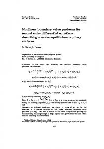
Figure 1. The solution at times t = 0.25 (left column), t = 0.75 (middle column), and t = 1.25 (right column) for b = 0 (top row), b = 0.5 (middle row), and b = i 0.5 (bottom row). The bottom row is showing the real part of the solution (u(1) ). It is also interesting to monitor the max norm of the solution for longer times when b = 0.5, see Figure 3. Note that the solution grows exponentially with time, illustrating the Unstable nature of this boundary condition. Also note that the solution is slightly larger on the finer grid. This behavior agrees with the predicted exponential growth proportional to |ω|t , because higher values of |ω| are captured on the finer grid. Note, however, that this growth is not due to numerical instabilities because the accuracy test shows second order convergence, at least up to t = 10, see Table 1. To more clearly see the difference between the cases b = 0 and b = i β we take F = 0, g0 = g1 = 0 and change the initial data to trigger a surface wave, f1 (x, y) = us (x, y, 0), where
f2′ (x, y) = us (x, y, −δt ),
� � �i h � p p us (x, y, t) = e−|βω0 |x cos ω0 (y − 1 − β 2 t) + i sin ω0 (y − 1 − β 2 t) ,
βω0 > 0.
(124)
This wave decays exponentially away from the x = 0 boundary with a harmonic oscillation pin y, see Figure 4. The surface wave propagates in the positive y-direction with a wave speed proportional to 1 − β 2 . As β → 0,
27
TITLE WILL BE SET BY THE PUBLISHER
Figure 2. The solution of the unstable case (b = 0.5) at times t = 2.5 to t = 4.5 in increments of 0.25, starting in the top left sub-figure and progressing row-wise to the bottom right subfigure, e.g. t = 2.75 is in the middle column of the top row.
4
10
2
10
0
10
2
4
6
8
10 Time
12
14
16
18
20
Figure 3. The max norm of the solution for 0 ≤ t ≤ 20 for the case b = 0.5, starting from a Gaussian pulse. The blue dots correspond to grid size h = 10−2 and the red crosses have h = 5 × 10⁻³ . the surface wave decays slower and slower in the x-direction. In the limit β = 0, the amplitude of the wave is
28
TITLE WILL BE SET BY THE PUBLISHER
constant in x which corresponds to one-dimensional wave propagation in the y-direction, consistent with the limiting boundary condition ux = 0. There are no numerical difficulties in this limit. 1
0.9
0.8
0.7
0.6
0.5
0.4
0.3
0.2
0.1
0
0
0.1
0.2
0.3
0.4
0.5
0.6
0.7
0.8
0.9
1
Figure 4. The real part of the initial data for the surface wave with β = 0.5 and ω0 = 8π. The case |β| → 1 is more difficult to solve numerically. Here we study 0.5 ≤ β < 1 and we use (124) as an approximation of the exact solution (us is only exponentially small at x = 1 and does not exactly satisfy the boundary condition at that boundary). To make sure the amplitude of the surface wave is negligible at the x = 1 boundary, we choose ω0 = 8π,
e−|βω0 | = e−4π ≈ 3.48 × 10⁻⁶ ,
β = 0.5.
In Table 2 we show the max norm of the error us − v for different values of β. The case β = 0.5 shows second order convergence, both at time t = 1 and t = 10. As can be expected in wave propagation problems, the error is dominated by the phase error, which explains why it is about 10 times larger at t = 10 compared to t = 1. For β = 0.9, the error still converges to second order accuarcy at time t = 1, but shows an unexpected pattern at time t = 10. Here the error is larger for the intermediate grid size h = 5 × 10⁻³ than for the coarse grid size h = 10−2 . This behavior is explained by studying the time history of the error, see Figure 5. For h = 10−2 , the max error occurs at t ≈ 5.5 when the numerical solution is about 180 degrees out of phase with the exact solution. At later times the error in the numerical solution decreases because it is between 180 and 360 degrees out of phase. The grid with h = 5 × 10⁻³ is barely fine enough to capture the solution at time t = 10 because the phase error exceeds 90 degrees. As a result we don’t see the expected second order convergence when the grid is refined to h = 2.5 × 10⁻³ . However, the error at t = 10 is about 10 times larger than at t = 1 for the finest grid, which indicates that this resolution is adequate for β = 0.9. The situation is even more dire for β = 0.99. Here the errors at time t = 1 show a simular behavior as at t = 10 for β = 0.9, so only the finest grid provides adequate resolution at t = 1. At t = 10, the error displays a completely erratic behavior with the
29
TITLE WILL BE SET BY THE PUBLISHER
largest error for the finest grid. An even finer grid would be necessary to obtain an accurate solution at t = 10, when β = 0.99. Case β = 0.5
h kus − vk∞ (t = 1) kus − vk∞ (t = 10) 1 × 10⁻² 2.44 × 10⁻² 2.38 × 10⁻¹ 5 × 10⁻³ 6.35 × 10⁻³ 6.19 × 10⁻² 2.5 × 10⁻³ 1.60 × 10⁻³ 1.56 × 10⁻² −2 −1 β = 0.9 1 × 10 6.04 × 10 2.46 × 10⁻¹ 5 × 10⁻³ 1.58 × 10⁻¹ 1.40 × 100 2.5 × 10⁻³ 4.00 × 10⁻² 3.95 × 10⁻¹ β = 0.99 1 × 10⁻² 1.67 × 100 1.37 × 100 −3 −1 5 × 10 5.20 × 10 1.81 × 10⁻¹ −3 −1 2.5 × 10 1.44 × 10 1.47 × 100 Table 2. Max error in the solution as function of the grid size when the exact solution is the surface wave us (x, y, t).
2 1.5 1 0.5 0
0
1
2
3
4
5
6
7
8
9
10
Figure 5. The max norm of the error as function of time for a surface wave with β = 0.9 computed on a grid with h = 10−2 (blue), h = 5 × 10⁻³ (green), and h = 2.5 × 10⁻³ (red). So why is it so hard to calculate an accurate numerical solution as |β| → 1? The spatial resolution in terms of grid points per wave length only depends on ω0 . With ω0 = 8π, the wave length is 1/4 and grid sizes h = 10−2 , 5 × 10⁻³ , 2.5 × 10⁻³ correspond to 25, 50, and 100 grid points per wave length, respectively. The exponential decay in the x-direction only depends weakly on β and never exceeds e−|ω0 |x for β < 1. Hence the solution varies on the same length scale in the x- and y-directions. Furthermore, the temporal resolution in terms of time steps per period only improves as |β| → 1 because the wave speed goes to zero in this limit. We conclude that the numerical difficulties are not due to poor resolution of the solution. To further analyze the cause of the poor accuracy in the numerical solution for |β| → 1, we decompose the problem (108)-(112) into two parts, u(x, y, t) = U (x, y, t) + u′ (x, y, t), such that U satisfies a doubly periodic problem on an extended domain, Utt = Uxx + Uyy + F˜ (x, y, t),
−1 ≤ x ≤ 2, 0 ≤ y ≤ 1, t ≥ 0,
subject to initial conditions, U (x, y, 0) = f˜1 (x, y),
Ut (x, y, 0) = f˜2 (x, y),
−1 ≤ x ≤ 2, 0 ≤ y ≤ 1,
30
TITLE WILL BE SET BY THE PUBLISHER
and periodic boundary conditions U (x, y, t) = U (x, y + 1, t), U (x, y, t) = U (x + 3, y, t),
−1 ≤ x ≤ 2, t ≥ 0, 0 ≤ y ≤ 1, t ≥ 0.
The interior forcing function and the initial data can be smoothly extended to become 3-periodic in the xdirection, without changing them on the original domain, F˜ (x, y, t) = F (x, y, t),
f˜k (x, y) = fk (x, y),
0 ≤ x ≤ 1, 0 ≤ y ≤ 1, t ≥ 0.
The problem for U is independent of the b-coefficient in the boundary condition and can easily be solved numerically. The difference u′ = u − U satisfies the scalar wave equation (108)-(112) with homogeneous interior forcing, homogeneous initial data, but inhomogeneuos boundary conditions, u′x − b u′y = g0′ (y, t) x = 0, 0 ≤ y ≤ 1, t ≥ 0, u′x
=
g1′ (y, t)
(125)
x = 1, 0 ≤ y ≤ 1, t ≥ 0,
(126)
The boundary forcing functions depend on U according to g0′ (y, t) = g0 (y, t) − (Ux (0, y, t) − b Uy (0, y, t)) , 0 ≤ y ≤ 1, t ≥ 0,
g1′ (y, t) = g1 (y, t) − Ux (1, y, t),
0 ≤ y ≤ 1, t ≥ 0.
The corresponding half-plane problems were analyzed in section 2.2. The accuracy problems are unlikely to arise from the Neumann boundary condition at x = 1 since it is independent of the b-coefficient. However, the half-plane problem subject to (125) satisfies the estimates of Theorem 2.8. Here, b = i β corresponds to case 2), and estimate (39) shows that the Laplace-Fourier transform of u′ satisfies |˜ u′ (0, ω, s)|2 ≤
g0′ |2 Cβ 2 |˜ , 1 − β 2 η2
Re s = η > 0,
(127)
p for (ω, s) in the vicinity of the generalized eigenvalue s0 = ±i 1 − β 2 ω0 . In general, the solution becomes unbounded as p |β| → 1. The truncation error terms which perturb the numerical solution are therefore amplified by a factor 1/ 1 − β 2 , which explains the poor accuracy in the numerical solution as |β| → 1. For boundary data g0 (y, t) which have a Laplace-Fourier transform that can be written as ˜ g˜0 (ω, s) = sG(ω, s), estimate (127) becomes |˜ u′ (0, ω, s)|2 ≤
˜2 ˜2 ˜2 Cβ 2 |s|2 |G| Cβ 2 |s|2 |G| |G| ≈ = Cβ 2 ω02 2 , 2 2 2 2 2 1−β η |s0 | /ω0 η η
s → s0 .
Hence the |β| → 1 singularity cancels out and the solution is bounded independently of β. The factor ‘s’ on the Laplace transform side corresponds to a time-derivative on the un-transformed side. Hence, the solution is bounded independently of β if the boundary forcing can be written as a time-derivative of a function with bounded Laplace-Fourier transform, Z 1 Z ∞ −2πiωy −st g0 (y, t) = Gt (y, t), G(y, 0) = 0, e e G(y, t) dtdy < ∞, Re s ≥ 0. y=0
t=0
31
TITLE WILL BE SET BY THE PUBLISHER
The latter condition is satisfied if G(y, t) is in L1 , i.e., Z
1
y=0
Z
∞ t=0
|G(y, t)| dtdy < ∞.
(128)
To test this theory numerically, we use a homogeneous interior forcing (F = 0) and homogeneous initial conditions (f1 = f2 = 0), homogeneous forcing on the x = 1 boundary (g1 = 0), and consider three different (1) (2) (3) forcing functions on the x = 0 boundary: g0 (y, t) = G(y, t), g0 (y, t) = Gt (y, t), and g0 (y, t) = Gtt (y, t). Here we choose G(y, t) to trigger a surface wave: 2
G(y, t) = us (0, y, t) e−(t/t0 −7) ,
t0 = 0.2,
where us is defined by (124). The Gaussian pulse exp(−(t/t0 − 7)2 ) decays exponentially fast away from its center at t = 7t0 . For example, it equals 1.23 × 10⁻⁴ at t = 7t0 ± 3t0 , and 5.24 × 10⁻²² at t = 7t0 ± 7t0 . The (2) (3) function G(y, t) satisfies (128), so our theory predicts that boundary forcings g0 and g0 should give solutions that are bounded independently of β. However, the time-integral of a Gaussian pulse is the error-function (erf), (1) so the boundary forcing g0 does not satisfy (128). In the numerical calculations we take ω0 = 8π and study the cases β = 0.5, β = 0.9, and β = 0.99. The grid size and time step are h = 2.5 × 10⁻³ and δt = 0.5h. The max norm of the solution as function of time is shown (1) in Figure 6. The case g0 = G in the top sub-figure illustrates the general case where the solution grows as p |β| → 1. Note that estimate (127) predicts the solution to grow like β/ 1 − β 2 , which means that the solution should be about 3.5 times larger for β = 0.99 than β = 0.9. In the numerical calculation, the max norm of the solution grows from about 0.75 for β = 0.9 to 3.75 for β = 0.99, which is slightly faster than predicted by theory. (3) The case g0 = Gtt in the bottom sub-figure shows the opposite situation when the solution decays as β → 1 because the forcing function is a second time-derivative of a function with bounded L1 norm, corresponding to (2) an s2 factor on the Laplace transform side. The intermediate case g0 = Gt is shown in the middle sub-figure. (1) Here the solution grows between β = 0.9 and β = 0.99, but not as fast as for gp 0 . To more closely study the behavior near β = 1, we take β = 0.995, 0.999 and 0.9997 corresponding to 1 − β 2 ≈ 0.0998, 0.0447 and 0.0244, respectively. To properly resolve the solution we here use an extra fine grid with h = 1.25 × 10⁻³ and δt = 0.5h. The max norm of the solutions, shown in Figure 7, reveal that the solution indeed stays bounded (2) independently of β, confirming our theory also for boundary forcing g0 = Gt .
Appendix In this appendix we collect a number of auxilary lemmas. Lemma A.1. The solution of yx = λy + F,
Re λ > 0,
0≤x 0. �
Lemma A.2. The solution of yx = −λy + F,
y(0) = g,
Re λ > 0,
0 ≤ x < ∞,
satisfies kyk2 ≤
1 1 kF k2 . |g|2 + Re λ (Re λ)2
(130)
33
TITLE WILL BE SET BY THE PUBLISHER
18 16 14 12 10 8 6 4 2 0 0
1
2
3
4
5 Time
6
7
8
9
10
Figure 7. The max norm of the solution as function of time for the boundary forcing function (2) g0 = Gt for β = 0.995 (blue/dots), β = 0.999 (red/diamonds) and β = 0.9997 (black/plusses). Proof. 2
As y ∈ L , integrating we have
hy, yix = 2Re hy, yx i = −2(Re λ)|y|2 + 2Re hy, F i. −|y(0)|2 = −2Re λ kyk2 + 2Re (y, F )
≤ −2Re λ kyk2 + 2 kyk kF k ≤ −2Re λ kyk2 + Re λ kyk2 +
Thus,
and the lemma follows.
Re λ kyk2 ≤ |y(0)|2 +
kF k2 . Re λ
kF k2 Re λ
√ √ Lemma A.3. Let a, b be real and consider a + ib with −π < arg(a + ib) ≤ π, arg z = following inequalities hold p p √ 2−1/4 |a| + |b| ≤ | a + ib| ≤ |a| + |b| p √ √ √ 2−3/4 | a + ib| ≤ 2−3/4 |a| + |b| ≤ Re a + ib ≤ | a + ib| for a ≥ 0, √ √ |b| |b| ≤ Re a + ib ≤ | a + ib| for a ≤ 0. ≤ 2−1 p 2−5/4 √ | a + ib| |a| + |b| √ Proof. In polar notation a + ib = ρeiθ , ρ = a2 + b2 > 0, −π < θ ≤ π, and
� 1 2 arg z.
Then, the (131) (132) (133)
√ θ √ a + ib = ρ ei 2
We have
p √ p √ |a| + |b| = ρ | cos θ| + | sin θ| ≥ 21/4 ρ and the first inequality in (131) follows. The second inequality in (131) follows from the triangle inequality. If a ≥ 0 then 2θ ∈ [−π/4, π/4] and (131) implies √ √ √ | a + ib| ≥ Re a + ib = ρ cos(θ/2) ≥
√ p √ 2 ρ ≥ 2−3/4 |a| + |b| ≥ 2−3/4 | a + ib| 2
34
TITLE WILL BE SET BY THE PUBLISHER
which is (132). To prove (133) notice that, as a ≤ 0,
therefore
√ |b| |b| ρ sin θ √ p = ρ 2 sin(θ/2) cos(θ/2) ≤ 2 Re a + ib ≤ √ = √ ρ | a + ib| |a| + |b| √ √ |b| 1 p ≤ Re a + ib ≤ | a + ib| 2 |a| + |b|
and the inequality follows from (131).
� √ For the forthcoming lemmata, we remind the reader that s = η + iξ, where η, ξ ∈ R, and κ = ω 2 + s2 . We shall now apply the last lemma to p κ = ω 2 + η 2 − ξ 2 + 2iξη, i.e., a = ω 2 + η 2 − ξ 2 , b = 2ξη. In the following three lemmas we denote by δ a constant with 0 < δ < 1.
Lemma A.4. Let Then
Also, always
√ δ1 = 2−1/4 δ,
δ2 = 21/2 (1 − δ)1/4 ,
( p δ1 ω 2 + |s|2 qp |κ| ≥ |s|2 + ω 2 η δ2
δ3 = min(δ1 , δ2 ).
if |ω 2 + η 2 − ξ 2 | ≥ δ(ω 2 + |s|2 ) otherwise.
|κ| ≥ δ3 η.
(134)
(135)
Proof. By (131) we obtain, for the first case, √ p p |κ| ≥ 2−1/4 |ω 2 + η 2 − ξ 2 | + 2|ξ|η ≥ 2−1/4 δ ω 2 + |s|2 . If |ω 2 + η 2 − ξ 2 | < δ(ω 2 + |s|2 ), then
2ξ 2 ≥ (1 − δ)(ω 2 + ξ 2 + η 2 ) = (1 − δ)(ω 2 + |s|2 ). Therefore −1/4
q √ p p 2|ξ|η ≥ 2 1 − δ ω 2 + |s|2 η.
|κ| ≥ 2 p 2 2 Also ω + |s| ≥ η implies (135). This proves the lemma. Lemma A.5.
Re κ ≥
(
2−5/4 |κ| √ 2 ω +|s|2 2−3/4 |κ| η
Re κ ≥ δ4 η,
if ω 2 + η 2 − ξ 2 ≥ 0,
if ω 2 + η 2 − ξ 2 < 0.
δ4 = 2−3/4 min(1, δ3 ).
Proof. If ω 2 + η 2 − ξ 2 ≥ 0, then (132) gives us Re κ ≥ 2−3/4 |κ| ≥ 2−3/4 δ3 η. If ω 2 + η 2 − ξ 2 < 0, then 2ξ 2 ≥ ω 2 + η 2 + ξ 2 = ω 2 + |s|2 . Therefore (133) gives us p ω 2 + |s|2 −3/4 −5/4 2|ξ|η ≥2 η ≥ 2−3/4 η. Re κ ≥ 2 |κ| |κ|
�
35
TITLE WILL BE SET BY THE PUBLISHER
This proves the lemma.
�
Lemma A.6. |κ| Re κ ≥ δ6
� � δ6 = min δ1 δ4 , 2−5/4 δ22 , 2−3/4 .
p ω 2 + |s|2 η,
Proof. If ω 2 + η 2 − ξ 2 ≥ 0, and |ω 2 + η 2 − ξ 2 | ≥ δ(ω 2 + |s|2 ), then (134) and (136) give us |κ| Re κ ≥ δ1
p ω 2 + |s|2 δ4 η.
If ω 2 + η 2 − ξ 2 ≥ 0, and |ω 2 + η 2 − ξ 2 | < δ(ω 2 + |s|2 ), then (134) and (136) give us |κ| Re κ ≥ 2−5/4 |κ|2 ≥ 2−5/4 δ22 Finally, if ω 2 + η 2 − ξ 2 < 0, by (136) we obtain |κ| Re κ ≥ 2−3/4 This proves the lemma.
p ω 2 + |s|2 η.
p |ω|2 + |s|2 η.
�
Lemma A.7. Assume that, for the boundary condition 1), a > 0, |b| < 1. Then there is a constant δ > 0 such that, for all ω and s with Re s ≥ 0, p |s + aκ − ibω| ≥ δ |s|2 + |ω|2 . For the proof, see Lemma 3 of [4]. Finally we have a lemma similar to Lemma A.4 and Lemma A.6 but for the normalized variables p κ′ = η ′2 − ξ ′2 + ω ′2 + 2iξ ′ ω ′ , ξ ′2 + ω ′2 = 1, |η ′ | ≪ 1.
By Lemma A.3,
p | − ξ ′2 + ω ′2 + η ′2 | + 2|ξ ′ | |η ′ | p Re κ′ ≥ 2−3/4 | − ξ ′2 + ω ′2 + η ′2 | + 2|ξ ′ | |η ′ | if ξ ′2 ≤ ω ′2 + η ′2 , |κ′ | ≥ 2−1/4
|ξ ′ |η ′ Re κ ≥ p | − ξ ′2 + ω ′2 + η ′2 | + 2|ξ ′ | |η ′ | ′
′2
′2
′2
if ξ > ω + η .
Lemma A.8. There is a constants δ > 0 such that |Re κ′ | ≥ δη ′ ,
|κ′ | ≥ 2−1/4 η ′ ,
|κ′ | |Re κ′ | ≥ δ6 η ′ .
where δ6 is that of Lemma A.6. Proof. From Lemma Lemma A.6, dividing by ω 2 + ξ 2 , p ω 2 + |s|2 |κ| Re κ η p ≥ δ6 p |κ | |Re κ | = 2 ≥ δ6 η ′ . 2 2 2 2 ω +ξ ω +ξ ω + ξ2 ′
′
Now if ω ′2 − ξ ′2 ≥ 0, then ω ′2 − ξ ′2 + η ′2 ≥ η ′2 , and p p |ω ′2 − ξ ′2 + η ′2 | + 2|ξ ′ |η ′ ≥ η ′2 + 2|ξ ′ |η ′ ≥ η ′ , so that, by Lemma A.3,
|κ′ | ≥ 2−1/4 η ′ ,
and Re κ′ ≥ 2−3/4 η ′ .
(136)
36
TITLE WILL BE SET BY THE PUBLISHER
If ω ′2 − ξ ′2 ≤ 0 then |ξ ′2 | ≥ 1/2. From (136) |κ′ | ≥ 2−1/4
q √ 2 2 η ′ ≥ 21/2 η ′ .
This last estimate also holds for |Re κ′ | when ω ′2 − ξ ′2 + η ′2 ≥ 0. When ω ′2 − ξ ′2 + η ′2 ≤ 0 we just use |ω ′2 − ξ ′2 + η ′2 | + 2|ξ ′ | η ′ ≤ const. and from (136) the estimate for Re κ′ follows from (136). This proves the lemma. � We thank Prof. Oscar Reula who participated in the original discussions leading to this work.
References [1] [2] [3] [4]
H.-O. Kreiss. Initial boundary value problems for hyperbolic systems. Commun. Pur. Appl. Math., 23:277–298, 1970. H.-O. Kreiss and J. Lorenz. Initial-boundary value problems and the Navier-Stokes equations. Academic Press, San Diego, 1989. B. Gustafsson, H.-O. Kreiss and J. Oliger. Time dependent problems and difference methods. Wiley-Interscience, 1995. H.-O. Kreiss and J. Winicour. Problems which are well posed in a generalized sense with applications to the Einstein equations. Class. Quantum Grav., 23(16):405–420, 2006. [5] M. S. Agranovich. Theorem on matrices depending on parameters and its applications to hyperbolic systems. Funct. Anal. Appl., 6:85–93, 1972.