Input Variable Selection: Mutual Information and Linear Mixing ...

JOURNAL OF LATEX CLASS FILES, VOL. 1, NO. 8, AUGUST 2002

1

Input Variable Selection: Mutual Information and Linear Mixing Measures Thomas Trappenberg, Jie Ouyang, and Andrew Back, Member, IEEE

Abstract— Determining the most appropriate inputs to a model has a significant impact on the performance of the model and associated algorithms for classification, prediction and data analysis. Previously we proposed an algorithm ICAIVS which utilizes independent component analysis (ICA) as a preprocessing stage to overcome issues of dependencies between inputs, before the data being passed through to an inout variable selection (IVS) stage. While we demonstrated previously with artificial data that ICA can prevent an overestimation of necessary input variables, we show here that mixing between input variables is common in real world datasets so that ICA preprocessing is useful in practice. This experimental test is based on new measures introduced in this paper. Furthermore, we extend the implementation of our variable selection scheme to a statistical dependency test based on mutual information and test several algorithms on gaussian and sub-gaussian signals. Specifically, we propose a novel method of quantifying linear dependencies using ICA estimates of mixing matrices with a new Linear Mixing Measure (LMM). Index Terms— Input variable selection, modeling, data preprocessing, independent component analysis, mutual information estimation.

I. I NTRODUCTION

I

NPUT variable selection is a simple concept: the idea is that of all the observed inputs from which we seek to develop a model for purposes such as classification, system identification, control, prediction etc, not all of them are essential to the model-building process. Moreover, if we include these unnecessary inputs, there may be noise introduced into the model, the parameter estimation process is made more difficult, and the overall results may be poorer than if only the required inputs are used. The area of input variable selection (IVS) has received renewed interest due to the increasing size of electronically available datasets [1], [2]. IVS is closely related to the well known area of feature selection. In the latter case, features may be informationbearing characteristics of a generative model or the observed data and may be spread across the space of inputs. Such features could also occur over time. There is usually a very specific method of extracting the features which is dependent on the generative model itself. In this paper, we consider the specific issue of selecting inputs, that is, given a data set x = [x0 ...xN −1 ]0 , how can we select a possible subset of indices IQ ∈ [0...N − 1] which yield, in some sense, the best or optimal performance for a given model and associated parameter estimation algorithm? This work was supported by NSERC Grant RGPIN 249885-03. T. Trappenberg is with Dalhousie University, Halifax, Canada J. Ouyang is with Oakland University, Rochester, USA A. Back is with Windale Technologies, Graceville,Australia.

This problem is not trivial and has been considered previously in various ways. What makes input variable selection a difficult problem is that, theoretically all possible subsets of inputs have to be considered in order to make an accurate decision about each input variable. While this problem might be unavoidable, it is possible that approximate solutions exploiting some heuristics can work well in practice. For example, forward or backward elimination schemes have been used traditionally for subset selection [3]. Most approaches depend statistically independent inputs, as this allows the IVS algorithms to perform various statistical tests to determine if an input index should be included1 in the set IQ . We have proposed previously an input variable selection algorithm known as ICAIVS [4] which has two distinct steps: 1) ICA: Taking the raw inputs, produce a set of “de-mixed” inputs which are as statistically independent as possible. 2) IVS: Perform a set of statistical tests between the demixed variables and the desired output variables. In our previous work we demonstrated that ICA preprocessing can reduce the overestimation of necessary inputs when inputs are linear mixtures of model dependent and independent variables. However, in order to claim that this preprocessing is useful in many applications we have to study how common mixing is in real world datasets. There appears to be a widespread belief within the data mining community that input variables are statistically dependent. For example, it has been shown that using combinations of input variables can result in more suitable representations for learning algorithms and hence improve performance in knowledge discovery and data mining applications [5], [6], [7]. However, no quantitative analysis has been made to our knowledge. Our objective here is to determine how likely it is in practice that such ICA demixing is required. To do this, we propose to perform a number of experiments on real world datasets. This will be addressed in the second part of this paper. In the first part of this paper we extend our implementation of the input variable selection scheme. Our previous selection was based on higher order cross cumulants to determine the dependence of each input on the desired output. However, there are various ways in which this dependence can be estimated. A popular choice is mutual information (MI) as a measure of dependencies, and in this paper we seek to determine the performance of a range of MI estimation methods in the input 1 In the discussion that follows, we will dispense with the notation and specific wording to indicate input indices. Instead it should be understood that when we say inputs, this implies the above indices context.

JOURNAL OF LATEX CLASS FILES, VOL. 1, NO. 8, AUGUST 2002

variable selection step. We compare these methods with our original cumulant-based method and a simpler correlationbased method. The paper is organized as follows. In Section II, we review several mutual information estimation methods that have been proposed in the literature. In Section III we perform some simulations to gauge the performance of various mutual information estimators. This approach is taken in an attempt to give an indication of the relative advantages and disadvantages of some basic methods for MI estimation that can be used for IVS. In Section IV, we then compare our original ICAIVS algorithm using equally weighted cumulants with the best MI estimators from the previous section. In Section V we propose a novel method of quantifying linear dependencies using ICA estimates of mixing matrices with a new Linear Mixing Measure (LMM). In Section VI we apply the proposed LMM to derive estimations of a mixing strength for several machine learning databases. II. E VALUATION OF A LGORITHMS FOR I NPUT VARIABLE S ELECTION A. Mutual Information for IVS Although many techniques can be proposed for IVS, MI can be seen as a very fundamental statistical approach to determine the dependence between variables. MI is a natural measure for selecting input signals, and such measures have been used previously for input variable selection [8], [9]. It is not always easy to find ways to reliably estimate MI, for example, it is well known in the statistical literature that a sufficient amount of data must be used to obtain valid results, whatever method is used. However, the task of using MI for selecting inputs is not the same as computing MI directly. Since we only require a relatively simple binary decision to be made about the dependence or otherwise of signals, it is not necessary to compute a precise value for the joint mutual information (JMI). This has formed the basis of the ICAIVS algorithm that was proposed previously [4]. In this case, higher-order cross cumulants were normalized and combined in a heuristic way to guide the decision process, without the precise value for mutual information ever needing to be estimated. In this section, we consider a number of MI estimation algorithms and seek to determine their suitability for input variable selection. B. Definition of Mutual Information For completeness, we include the definition of MI and JMI. Shannon’s definition of MI between an input signal x and output signal y is given as the Kullback-Leibler distance between the joint PDF f (x, y) and the product of the marginal PDFs f (x) and f (y), Z ∞Z ∞ f (x, y) )dxdy. (1) I(x, y) = f (x, y) log( f (x)f (y) −∞ −∞ Statistical dependencies between subsets of input signals and an output signal can similarly be defined as the JMI, for

2

example

Z

∞

Z

Z

∞

∞

I(x1 , x2 , y) =

f (x1 , x2 , y) −∞

−∞

−∞

f (x1 , x2 , y) )dx1 dx2 dy f (x1 , x2 )f (y) I(x1 , y) + I(x2 , y|x1 ) × log(

=

(2) (3)

C. Mutual information estimation methods Bonnlander and Weigend compared two MI estimation methods, one based on PDF estimations with a kernel method and one which is based on PDF estimations with an equalmass binning method [8]. The experimental results show that the estimated value for MI depend highly on the choice of algorithmic parameters such as the kernel width and bin width. However, kernel width and bin width did not change the rank of the relevance of the input subsets for reasonable parameters. Yang and Moody proposed another method to estimate JMI, I(xi , xj , y), i 6= j, for data visualization [9]. For the purpose of data visualization, the two most important inputs were selected. The JMI methods take advantage of using conditional MI to rank combinations of two input variables when the MI of individual inputs (e.g. I(xi , y)) is the same. In this paper we compare some further methods of MI estimation. This includes a standard (equal bin) histogram method (HG), an adaptive partitioning histogram method (AP) proposed by Darlellay and Vajda [10], and MI estimation based on the Gram-Charlier polynomial expansion (GC) [11]. The AP histogram method is similar to the histogram methods used by Bonnlander and Weigend in that it aims at partitioning the range of random variables into bins containing the same number of samples, so that the influence of each bin is balanced. Unlike the binning method used in [8], the AP partitioning is a recursive method that subpartitions the space based on an χ2 to test if the current data distribution is close to uniform. The GC method of MI estimation is based on the GramCharlier polynomial expansion of a PDF [11], f (x) ∼

∞ X n=0

cn

dn Z(x) , dxn

(4)

2

/2) √ where Z(x) = exp(−x is a gaussian function and cn are 2π factors that determine the weights of different order derivations of Z(x). Using the truncated polynomial expansion for marginal PDFs, Amari et al. [12] derived an approximation of the marginal entropy

(k x )2 5 · (k3x )2 k4x (k x )3 2eπ (k3x )2 ˆ − − 4 + + 4 . (5) H(x) = 2 2 · 3! 2 · 4! 8 16 Here k3x and k4x are 3rd and 4th order cumulants that can be calculated from moments mxn = E(xn ) as k3x = mx3 , k4x = mx4 − 3. Using the fourth order Gram-Charlier expansion for two-dimensional joint PDF, Akaho et al. [13] derived the joint entropy 1 (6) H(x, y) = H(r, s) + log (1 − ρ2 ) 2

JOURNAL OF LATEX CLASS FILES, VOL. 1, NO. 8, AUGUST 2002

3

where ρ = E[xy], r and s are a linear combination of x and y (assumed to be zero mean and unit variance), · ¸ µ + −¶ · ¸ r c c x = (7) s c− c+ y c+

=

c−

=

(1 + ρ)−1/2 + (1 − ρ)−1/2 2 (1 + ρ)−1/2 − (1 − ρ)−1/2 , 2

(8) (9)

and

x and y have the same distribution with zero mean and variance equal to 2. The two signals are dependent on each other as the joint PDF is not equal to the product of marginal PDFs. To generate this data set, we generated random numbers according to f (x, y) with a two-dimensional Metropolis algorithm [16]. The MI for this example can be calculated analytically from eq.1. For the second data set, the dependent sub-gaussian signals are generated from two independent sub-gaussian signals f (x) = f (y) =

ˆ s) = H(r,

12x2 (1 − x), 0 ≤ x ≤ 1 2y, 0 ≤ y ≤ 1

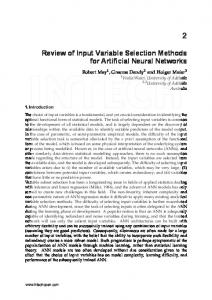
1 + log 2π 1 f (x, y) = 24x2 (1 − x)y, 0 ≤ x, y ≤ 1, (13) − [(β3,0 )2 + 3(β2,1 )2 + 3(β1,2 )2 + (β0,3 )2 ] 2 · 3! where each of the random numbers X and Y are generated 1 − [(β4,0 )2 + 4(β3,1 )2 + 6(β2,2 )2 + 4(β1,3 )2 + (β0,4 (10) )2 ] with a standard Metropolis algorithm [17]. To make the desired 2 · 4! dependent signals, we generate two new signals that are where functions of the independent signals. The new signals are: · ¸ µ ¶· ¸ βk,l = E{rk sl } − β0k,l  u 1 C x = , (14)  3 k=4 or l=4 v C 1 y k,l 1 k=l=2 β0 = µ ¶  1 C 0 otherwise. where is a covariance matrix and C is a covariance C 1 The MI can then be calculated from these estimates as parameter. The strength of the dependency between u and v ˆ ˆ ˆ ˆ I(x, y) = H(x) + H(y) − H(x, y), (11) can be adjusted by tuning the value of C. Thus, by changing the covariance between u and v we also change the value which corresponds to a polynomial of high order cumulants. of MI. The joint PDF f (u, v) of the dependent sub-gaussian While there are other choices to measure the difference signals can be calculated with a coordinate transformation between statistical distributions [14] on which a statistical taking the Jacobian into account, and is given by dependency test can be based, MI has become a benchmark (Cv − u)2 (Cu − v)((Cv − u)/(C 2 − 1) − 1) of choice for IVS. f (u, v) = 24 . (C 2 − 1)4 (15) III. P ERFORMANCE OF M UTUAL I NFORMATION The theoretical value for MI can then be calculated by numerE STIMATORS ical integration. In this section we describe the results of a number of experiments on different MI estimation methods. We consider B. Experimental Results two data sets: a set of two dependent gaussian signals, and a We conducted a range of experiments on the MI estimation mixture of two independent sub-gaussian signals. algorithms described above. Specifically, we examined the While in the literature many performance tests of MI esdependence of the MI estimation for different numbers of timators are made with independent signals, we think that training samples and also calculated the averages and standard tests on dependent signals are important. The aim of the deviations over 20 runs2 . The results of the MI estimations of experiments reported here is to carefully control the degree the gaussian signals are shown in Figure 1. All three estimation to which dependence is introduced between variables. An methods gave reasonable estimates of the theoretical MI important aspect of the experiments is that we can calculate (dotted line) with enough data points in the sample, although the theoretical value for the MI between signals in order to the AP method converged first. The results for the sub-gaussian assess their accuracy. signals with covariance parameter C = 0.2 and C = 0.6 are shown in Figure 2. A. Experimental Data For the first data set we use gaussian distributions with the following PDFs [15] f (x)

=

f (y)

=

f (x, y)

=

x2 1 √ e− 4 , −∞ < x < ∞ 2 π y2 1 √ e− 4 , −∞ < y < ∞ 2 π √ 3 − (x2 −xy+y2 ) 3 e , −∞ < x, y < ∞. (12) 6π

C. Discussion of the experimental results In these experiments the AP estimator demonstrated outstanding performance. For each single test with different C, the AP estimator converges to the analytical value after a certain 2 Most estimation methods depend on some algorithm specific parameters such as the bin width in HG and the partitioning threshold in AP. We attempted to choose these parameters fairly for each case to give a true representation of the performance of each algorithm.

JOURNAL OF LATEX CLASS FILES, VOL. 1, NO. 8, AUGUST 2002

4

Test on Gaussian Signals

Estimated mutual information

0.18 0.17 0.16 0.15 0.14 0.13 0.12

Analytical Value GC AP HG

0.11 0.1 0.09 100

1090 2080 3070 4060 5050 6040 7030 8020 9010 10000

Number of Samples Fig. 1. Estimation accuracy of three MI estimators on gaussian signals with varying number of sample points.

D Estimated Mutual Information

0.6

Test on Sub−Gaussian Signals (C=0.2) Analytical Value GC AP HG

0.5 0.4 0.3 0.2 0.1

IV. ICAIVS: E QUALLY W EIGHTED C UMULANTS OR M UTUAL I NFORMATION ?

0 −0.1 −0.2 100

2080

4060

6040

8020

10000

Number of Samples

E

1

Test on Sub−Gaussian Signals (C=0.6)

0.95

Estimated Mutual Information

number of samples. As the MI increases, the required number of samples increases. The HG estimator performs similarly to the AP estimator when the dependence between the signals is not very high (Figure 2a). However, the HG estimate exhibits a systematic shift when the MI increases to a certain level, although the bin width was tuned appropriately. The deviation between the theoretical value and the estimate becomes larger as the MI increases. Thus, testing the methods on independent signals would not have revealed this difference. The GC estimator experienced difficulty converging and systematically underestimated the theoretical value in all subgaussian tests. The comparison of these three MI estimators can be summarized as follows: The advantage of MI estimation with GramCharlier expansion is that it only calculates the expectation value of different powers of the samples. Thus it is fast and easy to calculate. The disadvantage of the GC method is that the estimate might suffer from the truncation of the expansion in the case of non-gaussian signals. This resulted in an underestimate of MI in our example of sub-gaussian signal, although the 4th order was taken into account in our implementation. The histogram based methods are in this sense more general than polynomial expansion based methods because they are less sensitive to the nature of the signals. However, the histogram methods are sensitive to the bin partitioning. A rough partition might result in bias toward high MI while finegrained partitions might result in underestimating MI. A good choice of bin width is particularly important for MI estimation as the regions with low data densities carry large information content (such as the tails of a distribution).

0.9 0.85 0.8 0.75 0.7

Analytical Value GC AP HG

0.65 0.6 0.55 0.5 100

2080

4060

6040

8020

Having determined the most appropriate MI estimator in the previous section, we ask - will the MI estimator give better performance than the original method of higher order equally weighted cross cumulants? In this section, we compare our original ICAIVS algorithm with a new version which employs MI. We choose to consider the two best performing MI estimation methods from the previous section, GC and AP, and for interest, a simple test based on a correlation measure to show the effect of higher order statistics. To keep the comparison results easy to understand, we report only the test results between individual input signals and the output signals. More complex tests between other subset combinations have also been considered, but are not included in the results reported here3 .

10000

Number of Samples Fig. 2. Comparison of performance of three different MI estimators on sub-gaussian data. Correlated signals are made with covariance parameter (a) C = 0.2 and (b) C = 0.6.

A. Experiment 1 For the first test we considered the example discussed in the original ICAIVS implementation [4]. This example consists of 3 For the mutual information estimation algorithms, we did not tune the partitionining parameters, instead we used the default partition of the algorithms.

JOURNAL OF LATEX CLASS FILES, VOL. 1, NO. 8, AUGUST 2002

15

0.5 0 −0.5

0

5 10 Input index

(d)

5 10 Input index

15

(c)

Correlation based ICAIVS 1

0.5

15

0 0

5 10 Input index

15

Fig. 3. Input variable selection results for the model of eqn. (16). Shown is the normalized dependency strength between the output value and each input value as estimated with (a) the equal-weight cumulant method, (b) the AP mutual information estimator, (c) the GC mutual information estimator, and (d) with correlation coefficients. Note that the choice of threshold in (a) is an open problem. In this case, we chose a nominal value. The difficulty in deciding relevant inputs in this case is evident.

15 iid signals x1 , ..., x15 normalized to be in the range −1 to 1. From these signals we used only the three signals x2 , x6 and x9 to generate the output signal based on the nonlinear model y = x32 + cos(x6 ) + 0.3 sin(x9 ).

(16)

To facilitate the comparison we show in the following normalized results in which each dependency value is divided by the largest value in the input set. Thus, the signal with the strongest dependency value has always a value of 1 (with exception of the data shown in Figure 4c). Figure 3 shows the results for the dependency values of the four methods. All methods identify the signals x2 and x9 with a considerable dependency strength, while the remaining dependent variable x6 is only identified by the AP method. The signal x6 is missed by the correlation method as the expectation value of x cos(x) is zero. Our results also indicate that such terms are difficult to detect with the cumulant and GC method.

B. Experiment 2 A further test is aimed at the case where the model is multiplicative between two signals, y = x2 ∗ x3 .

(17)

In this model, neither of the two inputs is dominant while only the product determines the output. The results are shown in Figure 4. The correct signals are identified by both MI methods, although the values of the MI in the GC method are all negative (no normalization was used in this sub-figure). A possible reason for the negative MI values is the underestimation mentioned before.

Estimated strength

0 0

1

0.8 0.6 0.4 0.2 0 0

5 10 15 Input Index Mutual Information (GC) based ICAIVS -0.02 -0.04 -0.06 -0.08 -0.1 -0.12

0

5 10 Input Index

0.8 0.6 0.4 0.2 0 0

5 10 Input Index Correlation based ICAIVS

(d)

15

1 Estimated strength

5 10 Input index

0.5

(b) Mutual Information (AP) based ICAIVS

Cross-Cumulant based ICAIVS 1 Estimated strength

0 0

(a)

1

Estimated strength

0.5

Mutual Information (GC) based ICAIVS 1 Dependecy strength

(c)

(b) Mutual Information (AP) based ICAIVS Dependecy strength

Dependecy strength

Cross−Cumulant based ICAIVS 1

Dependecy strength

(a)

5

15

0.8 0.6 0.4 0.2 0 0

5 10 Input Index

15

Fig. 4. Results for the input variable selection test for the model of eqn. (17). The normalized dependency strength between the output value and each input value as estimated with (a) the equal-weight cumulant method, (b) the AP MI estimator, (c) the GC MI estimator, and (d) with correlation coefficients (as in Figure 3). The maximum dependency strength in (c) is not normalized to a maximum of one because all numerical values are below zero. Note again the that the threshold in (a) is nominal value which presents some difficulties in deciding relevant inputs for this case.

C. Summary These simple experiments indicate that inputs can be detected by all the methods in some cases. For some situations, it can be difficult to detect the inputs reliably with the cumulant and GC method. The AP MI estimator offers evidently very good performance. This method also gave the best estimations of MI in our previous tests indicating that a more accurate estimation of MI can contribute to the accuracy of the IVS test. V. D O WE NEED TO USE ICA?: D EPENDENCE E STIMATION USING LMM S A. Linear Mixing Measures In this section we propose an efficiently computed measure we term LMM (Linear Mixing Measure) which quantifies the degree of mixing between input variables. This measure will be used to explore and quantify mixing between input signals in several machine learning datasets. There are a number of variations of LMMs that will be discussed in addition. For the discussion that follows, it is assumed that there is a set of inputs s that is passed through a mixing matrix M to give a set of mixed input variables x, x = Ms,

(18)

where M is a generally unknown, instantaneous mixing matrix, s is a vector of unobserved independent source signals, and x is a vector of observed dependent signals. In this scenario, x corresponds to the observed input data. We would like to determine how likely it is that ICA preprocessing for IVS, which corresponds to performing IVS on s, will have an effect on the results. A fully diagonal square mixing matrix M corresponds to zero mixing between source signals s. We require a criterion which measures the effect of off-diagonal elements in M that will result in signals being mixed. It is also necessary to estimate

JOURNAL OF LATEX CLASS FILES, VOL. 1, NO. 8, AUGUST 2002

the mixing matrix using ICA. The resulting estimate of the mixing matrix is denoted by A in the following. A is only an estimate of M up to column permutations and scaling factors of the individual signals which has to be taken into account in the definition of LMM. B. A Lower Bound on an LMM We define the LMM, E1C , as the sum of all elements of the matrix A minus the largest element of each column, where à n ! n X X 1 |aij | C E1 = −1 (19) n(n − 1) j=1 i=1 maxk |akj | and aij is an element of matrix A in the ith row and jth column. The superscript ‘C’ of this measure indicates that the normalization and inner summation is carried out over the columns of the matrix. E1C does not depend on either column or row permutations and can be calculated in quadratic time (O(n2 )). Remarks 1) The subscript 1 indicates that this measure is based on a linear weighting of the off diagonal elements. Other forms can be used, such as a square of the linear distances. 2) An appropriate definition of the total linear mixing based on the true mixing matrix can be defined as à n ! n X X 1 |mij | |mjj | M E1 = − , n(n − 1) j=1 i=1 maxk |mkj | maxk |mkj | (20) where mij are the elements of the (typically unknown) mixing matrix M. E1M measures the normalized4 sum of the differences between the normalized off-diagonal mixing strength and the normalized on-diagonal mixing strength. It gives an indication of the degree to which inputs are mixed, but does not take into account permutations of the input signals which E1C does. 3) Another LMM that we could have considered is © ª E1min = min E1M (B)|B ∈ Pc (A) (21) where Pc (A) is a set of all matrices resulting from all possible column permutations of A. This measure captures the main objective of the study to give a conservative estimate of mixing in real world datasets. However, while E1min overcomes the issue of permutations of the input signals, it has the disadvantage that it scales factorially due to the necessary permutations of A. 4) Another approach is to find the minimal mixing condition corresponding to the matrix B ∈ Pc (A) in which the sum of the diagonal elements is maximal. 4 Note that normalization is used here so that different mixing matrices can be compared, where only the relative magnitude of the off-diagonal elements to the diagonal elements are important. We also take normalization with respect to the rank n of the matrix into account so that the possible values of this strength measure range between 0 and 1 for mixing problems with arbitrary number of signals n.

6

This matrix is easy to find in the case that each column vector has the maximum value at a position different from the position of the maximum values in all the other column vectors. The matrix can then be found by placing each column vector at the position of the index of the maximal element. This ordering can be done in quadratic time (O(n2 )). The case when two column vectors from one mixing matrix have maximal elements at the same index is termed a coincident column maximum index. For any given matrix A, the index of the maximum value of column k is αk , k = 1, ..., n, we define Nc as the number of coincident column maximum indices where Nc

=

n X

ui

i

½ ui

=

x−1 0

when index i occurs x > 1 times (22) elsewhere.

It is not practical to try to find a measure of minimal mixing using an exhaustive search, testing all permutations of columns which have coincident column maximum indices. It is easy to see that E1C is a lower bound of E1min . The measure E1C is equal to E1min if A has no coincident column maximum indices because then the maximal element, which is 1 after normalization, can be placed on the diagonal with the ordering of the columns. If A has Nc > 0, then the above measure corresponds to the case of ignoring the coincident column maximum indices and allowing each column vector to be optimally placed with the maximal element on the diagonal. This introduces an error for each but one coincident column maximum index, underestimating the true mixing strength because a value of one instead of a true diagonal element less than one is subtracted from the sum of all elements of the column vector in the measure E1C . In other words, compared to the measure E1min , where the true diagonal element is subtracted, an error of 1 − aii is made for each but one coincident column maximum index, where aii is the diagonal element of the permutated matrix with the smallest mixing strength. A large value of E1C indicates a large value of E1min so that this measure is sufficient for our argument if E1C is large. However, a small value of E1C can still be caused by matrices with large E1min in the case where Nc is large. C. LMM with Column/Row Normalization We define the quantity E1R ,   n n X X 1 |aij |  E1R = − 1 , n(n − 1) i=1 j=1 maxk |aik |

(23)

which is similar to E1C except that the normalization is performed on the row vectors of the matrix A. E1R is also independent of permutations, and in case of Nc = 0 it holds that E1R = E1C = E1min . In the case of Nc > 0, E1R is an

JOURNAL OF LATEX CLASS FILES, VOL. 1, NO. 8, AUGUST 2002

7

0 .1 4

upper bound on E1min . As E1C is a lower bound on E1min , and E1R is an upper bound, it is appropriate to take the average (24)

as an approximation of E1min . This quantity corresponds to the measure E1 introduced by Amari et al. [12] up to a 1 normalization factor n(n−1) . A better LMM can be obtained by replacing the term E1R in the above definition with an estimate that performs the row normalization after a column normalization. The normalized LMM is defined by E1N

¢ 1¡ C E1 + E1CR , = 2

where the column/row-normalized LMM is given by   n n X X 1 |˜ aij |  E1CR = − 1 n(n − 1) i=1 j=1 maxk |˜ aik |

(25)

0 .1

Estimation error

¢ 1¡ C E + E1R E1 = 2 1

M

E 1R - E 1

0 .1 2

M

0 .0 8

E 1CR- E 1

0 .0 6

M

E 1- E 1

0 .0 4

M

E 1N - E 1

0 .0 2 0 -0 .0 2

M

E 1C - E 1

-0 .0 4 0

5

10

15

20

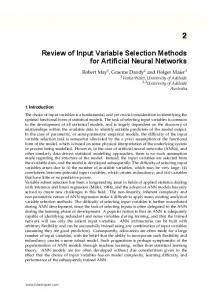
Nc Fig. 5. Example of LMMs from experiments with random mixing matrices with different numbers of coincident column maximum indices. As argued in the text, E1C is a lower bound on E1min and thus also smaller than E1M . E1N is the best estimate of E1M from all considered LMMs. All LMMs show a linear dependence on Nc in this example.

(26)

in which a ˜ij is an element of the column-normalized matrix µ ¶ aij ˜ = A . (27) maxk |akj | The measure E1N is very similar to the measure E1 introduced by Amari et al. [12]. However, note that E1 is most commonly used in the performance evaluation of ICA algorithms where the true mixing matrix is known. Here we adapted this criteria to the situation where the true mixing matrix is unknown. We augmented the original measure with a normalization factor to enable the comparison of mixing strength values between mixing matrices of different size. Note that E1 and E1N are the same when the columns of the estimated mixing matrix are first normalized. The different LMMs are illustrated with an example in Figure 5. Shown there is the average numerical values for the difference of the LMMs to E1M on random mixing matrices for different values of number of coincident column maximum indices Nc . In each experiment a random mixing matrix of size 21 × 21 with elements drawn equally between 0 and 1 was added to a unit matrix. This corresponds to a mixing matrix where Nc = 0. To generate mixing matrices where Nc > 0 we randomly picked a specific number of columns equal to Nc and exchanged the diagonal elements with the first element in the same column. Remarks 1) All the measures agree when Nc = 0. However, the quality of the approximation of E1M is different for increasing Nc . 2) In our experiments, E1C always underestimates the true value in case of Nc > 0, and this difference increases linearly with Nc . 3) E1R always overestimates E1M , and the difference from E1M increases with Nc . 4) E1 slightly overestimates E1M but is a reasonable approximation of E1M .

5) The best estimate of E1M when Nc > 0 is the measure E1N . 6) The minimal mixing strength, E1min , is always smaller or equal to E1M . The measure of E1N is thus overestimating E1min . However, as mentioned above, E1C is always a lower bound on E1min . Thus, E1C might overestimate the number of cases with small mixing strength, while E1N might underestimate the cases with small mixing strength. We are using therefore both measures, E1C and E1N , in the following study as the combination of these measures can provide a better picture of the possible range of expected mixing strength values.

VI. E XPERIMENTAL R ESULTS OF LMM S

A. How common are Dependent Inputs in Real World Datasets? Several datasets were chosen arbitrarily from four data collections, the StatLib-Datasets Archive [18], the Delve library [19], the UCI Machine Learning Repository [20], and the FMA collection [21]. These datasets stem from a variety of subject areas such as economics, robotics, or health informatics. The datasets present a good test of LMMs as the number of inputs range from 2 up to 33, and the number of samples range from tens to thousands (see Table I). For simplicity we omitted datasets with missing data and non-numeric feature values. In the remaining datasets we eliminated features which had no obvious problem-dependent meaning such as serial numbers, or which had obvious dependencies on other features such as classification numbers. To verify the stability of the LMM estimates with respect to the size of the samples, we calculated the mixing strength E1N

JOURNAL OF LATEX CLASS FILES, VOL. 1, NO. 8, AUGUST 2002

8

TABLE I R ESULTS OF THE ICA ANALYSIS FROM 30 DATASETS FROM PUBLIC MACHINE LEARNING DATASETS SPECIFIED IN THE TEXT. T HE MEASURED N , E C , AND N , ARE THE AVERAGE VALUES OVER 30 QUANTITIES E1 c 1 RUNS WITH DIFFERENT INITIALIZATIONS OF THE ICA ALGORITHM .

2

(100) (x)/E N EN 1 1

omitted dataset 1.5

P LEASE REFER TO THE TEXT FOR DETAILS OF THE DATASETS .

1

0.5

25

50

75

100

x (percentage of training data) Fig. 6. The dependency of E1N on the amount of training data used for the estimation in each of the 31 datasets. E1N is plotted for different values relative to the value as estimated from the complete dataset.

for different fractions of data5 . This is shown in Figure 6. Each curve represents the average of 30 trials. A steady value for large coverage was taken as an indication for convergence of the estimation. All but one dataset showed consistent values when most of the data was included, establishing some confidence that the number of samples is sufficient to estimate the mixing matrix. Only one dataset showed a strong variation of E1N for high percentages of the data. This dataset was not included in the following analysis. The detailed results of the estimates of E1C and E1N are given in Table I. In some problems it became evident that there are inputs supplied in the datasets that have no bearing on the technical problem. For clarity, these inputs were removed manually before commencing the experiments. The results for Nc and the various mixing strength measures represent averages over 30 trials with different starting conditions of the ICA algorithm. A histogram of values E1C , which represent a strict lower bound on the minimal mixing strength E1min , is shown in Figure 7 (open bars). 24 out of the 30 datasets have a lower bound of the mixing strength larger than 0.025, while half of the dataset have values of E1C larger than 0.075. We then compared the histogram of mixing strength estimations derived from E1C to the histogram of mixing strength estimation derived from E1N in Figure 7 (solid bars). With this estimate there are now 28 out of the 30 datasets with an estimated mixing values larger than 0.025 and 23 out of 30 with estimated mixing strength larger than 0.075. Interestingly, all of the 7 datasets with E1N < 0.075 are from 5 Datasets 1-17 are from the StatLib library [18], specifically (1) alr56, (2) alr57, (3) Boston house-price, (4) Body fat, (5) S&P Letters Data, (6) ch10, (7) ch17, (8) ch1a, (9) ch3a, (10) Wages, (11) Disclosure, (12) Irish Educational Transitions, (13) papir, (14) places, (15) pollen, (16) pollution, and (17) Child witness example. Datasets 18-25 are from the Delve library [19], specifically (18) KINematics-32fh, (19) KINematics-32fm, (20) KINematics-8fh, (21) KINematics-8fm, (22) PUMA DYNamics-32fh, (23) PUMA DYNamics32fm, (24) PUMA DYNamics-8fh, (25) PUMA DYNamics-8fm. Datasets 26-28 are from the the UCI library [20], specifically (26) Liver-disorders Database, (27) Iris Plants Database, and (28) Wine recognition data. Datasets 29 and 30 are from the FMA library [21], specifically (29) Bank Data, and (30) Boston Stock.

SN # Features # Samples # Nc 1 11 26 8.2 2 11 32 7.9 3 16 506 12.7 4 15 252 10.7 5 9 20640 7.9 6 7 60 1.1 7 13 68 11.9 8 4 704 3 9 4 50 0.9 10 11 534 7.1 11 4 662 3 12 6 500 4 13 13 29 4.3 14 9 329 5 15 5 481 2 16 16 60 14 17 14 42 5.4 18 33 8192 0 19 33 8192 0.3 20 9 8192 0.4 21 9 8192 1 22 33 8192 11.1 23 33 8192 13.8 24 9 8192 2 25 9 8192 1.6 26 6 345 1.4 27 4 126 2 28 13 138 11.4 29 3 60 2 30 2 35 1

E1N 0.28 0.31 0.16 0.23 0.16 0.44 0.11 0.24 0.5 0.21 0.16 0.28 0.42 0.27 0.42 0.11 0.44 0.02 0.02 0.03 0.1 0.05 0.06 0.04 0.06 0.2 0.52 0.11 0.29 0.37

E1C 0.19 0.22 0.07 0.16 0.03 0.44 0.04 0.05 0.49 0.16 0 0.21 0.41 0.21 0.39 0.03 0.43 0.02 0.02 0.03 0.09 0.05 0.05 0.03 0.04 0.17 0.42 0.02 0.03 0.2

simulated robotics experiments. The features in these datasets represent well designed measurements so we expect minimal dependency between inputs of these datasets. VII. D ISCUSSION AND C ONCLUSIONS MI is a valuable method that can be applied to input variable selection, both from a theoretical and practical point of view. In this paper, we have compared a range of MI algorithms and shown that the adaptive partitioning (AP) histogram method by Darlellay and Vajda [10] showed superior performance in our examples. The MI estimation method based on the Gram-Charlier expansion (GC) is also useful for input variable selection. Although this method does not provide very accurate MI values for data that are far from gaussian, some dependent signals were, nevertheless, detected with less computational effort compared to AP. We have shown that both MI estimation methods offer superior performance in terms of accuracy over the original higher order, equally weighted cross cumulant algorithm used in the original ICAIVS implementation [4]. In addition, the AP algorithm drastically simplifies the choice of threshold value for the final binary decision, since the values for the irrelevant data have also a very small value, whereas this was a problem in the previous method.

JOURNAL OF LATEX CLASS FILES, VOL. 1, NO. 8, AUGUST 2002

9

10

of highly redundant signals. This parallels to some extent the effect of ICA preprocessing. The results shown in this paper confirm that their approach should be highly relevant to many applications.

Number of datasets

8

6

R EFERENCES

4

2

0

0

0.1

0.2 0.3 0.4 E C1 (open bars), E N (solid bars) 1

0.5

Fig. 7. Distribution of E1C (open bars), which is a lower bound on the minimal possible mixing strength, and E1N (solid bars), which is a better estimate on the minimal possible mixing strength, in 30 real world datasets.

A further advantage of the MI methods compared to the cumulant method is that the values for the dependency indicator are more meaningful compared to the cumulants used in the original ICAIVS implementation. For example, the values for the MI can be used to rank the relative strength of the signals and to use this in the decision process to add additional inputs to the set of selected inputs. Such information could also be used to provide guidance in further model development. A disadvantage of the histogram based MI method is that it still suffers from the curse of dimensionality in that highdimensional histograms have to be evaluated when subsets of input variables are investigated. The GC method uses MI estimation based on the Gram-Charlier polynomial expansion of a PDF and hence this enables us effectively determine the orders of input variables to include. The LMMs introduced in this paper can be used to systematically quantify dependencies between signals from ICA estimates of mixing matrices. The application of LLM to several real world datasets demonstrates that ICA is a useful preprocessing step. While we demonstrated previously with artificial data that ICA can prevent an overestimation of necessary input variables, we show here that mixing between input variables is common in real world datasets, as demonstrated in a number of real world datasets. This indicates that ICA preprocessing is useful in practice to isolate the ”true” statistically independent data inputs from what can often be datasets with strong statistical dependencies between inputs. It seems important therefore, to ensure that preprocessing of data with ICA is available as part of any tool kit, including data mining. While completing this paper we became aware of a recent paper by Chow and Huang [22] who developed a new MI method for IVS based on similar points raised in this and our previous paper, that a precise estimation of MI is not necessary for a binary IVS decision step. This new method seems specifically promising in overcoming the dimensionality problem in MI estimation. Also, their IVS scheme includes the evaluation of MI between input signals to prevent the inclusion

[1] Ron Kohavi and George H. John. Wrappers for feature subset selection. Artificial Intelligence, 97(1-2):273–324, 1997. [2] Isabelle Guyon and Andr´e Elisseeff. An introduction to variable and feature selection. Journal of Machine Learning Research, 3:1157–1182, March 2003. [3] George H. John, Ron Kohavi, and Karl Pfleger. Irrelevant features and the subset selection problem. In International Conference on Machine Learning, pages 121–129, 1994. Journal version in AIJ, available at http://citeseer.nj.nec.com/13663.html. [4] Andrew D. Back and Thomas P. Trappenberg. Selecting inputs for modeling using normalized higher order statistics and independent component analysis. IEEE TRANSACTIONS ON NEURAL NETWORKS, 12(3):612–617, May 2001. [5] L.A. Rendell and R. Seshu. Learning hard concepts through constructive induction: Framework and rationale. Computational Intelligence, 6(4):247–270, 1990. [6] A.A. Freitas. Understanding the crucial role of attribute interaction in data mining. Artificial Intelligence Review, 16(3):177–199, November 2001. [7] Sylvain L´etourneau. Identification of Attribute Interactions and Generation of Globally Relevant Continuous Features in Machine Learning. PhD thesis, School of Information Technology and Engineering, University of Ottawa, Ottawa, Ontario, Canada, August 2003. [8] B. V. Bonnlander and A. S. Weigend. Selecting input variables using mutual information and nonparametric density estimation. In Proc. of the 1994 Int. Symp. on Artificial Neural Networks (ISANN”94), pages 42–50, Tainan, Taiwan, 1994. [9] Howard Hua Yang and John E. Moody. Data visualization and feature selection: New algorithms for nongaussian data. In T.K. Leen S.A. Solla and K.-R. Muller, editors, in Advances in Neural Information Processing Systems, volume 12. MIT Press, 2000. [10] Georges A. Darbellay and Igor Vajda. Estimation of the information by an adaptive partitioning of the observation space. IEEE Transactions on Information Theory, 45(4):1315–1321, May 1999. [11] S. Blinnikiov and R. Moessner. Expansions for nearly gaussian distributions. Astron. Astrophys. Suppl. Ser., 130:193–205, 1998. [12] S. Amari, A. Cichocki, and H. H. Yang. A new learning algorithm for blind signal separation. In David S. Touretzky, Michael C. Mozer, and Michael E. Hasselmo, editors, Advances in Neural Information Processing Systems, volume 8, pages 757–763. The MIT Press, 1996. [13] Shotaro Akaho, Yasuhiko Kiuchi, and Shinji Umeyama. Mica: Multimodal independent component analysis. Proc. of IJCNN, 1999. [14] S. Amari and H. Nagaoka. Methods of Information Geometry. AMS and Oxford University Press, 2000. [15] Enders A. Robinson. Probability Theory and Applications. International Human Resources Development Corporation, 1985. [16] Jie Ouyang. Improved icaivs algorithm with mutual information. Master’s thesis, Dalhousie University, 2004. [17] Siddhartha Chib and Edward Greenberg. Understanding the metropolishastings algorithm. The American Statistician, 49(4):327–335, November 1995. [18] Statlib—datasets archive, http://lib.stat.cmu.edu/datasets/. [19] Carl Edward Rasmussen, Radford M. Neal, Geoffrey Hinton, Drew van Camp, Michael Revow, Zoubin Ghahramani, Rafal Kustra, and Rob Tibshirani. Data for evaluating learning in valid experiments. [20] C.L. Blake and C.J. Merz. UCI repository of machine learning databases, http://www.ics.uci.edu/∼mlearn/mlrepository.html, 1998. [21] Spyros G. Makridakis, Steven C. Wheelwright, and Rob J Hyndman. Forecasting: Methods and Applications (3rd edition). John Wiley & Sons, 1998. [22] T.W.S. Chow and D. Huang. Estimating optimal feature subsets using efficient estimation of high-dimensional mutual information. IEEE TRANSACTIONS ON NEURAL NETWORKS, 16(1):213–224, 2005.

JOURNAL OF LATEX CLASS FILES, VOL. 1, NO. 8, AUGUST 2002

Thomas Trappenberg studied at RWTH Aachen University and held research positions in KFA/HLRZ J¨ulich, the RIKEN Brain Science Institute and Oxford University. He is currently associate professor in the Faculty of Computer Science at Dalhousie University and director of the graduate program in electronic commerce. His principle research interests are computational neuroscience and applications of machine learning methods for data classification and signal analysis. He is the author of the textbook ‘Fundamentals of Computational Neuroscience’ published by Oxford University Press.

Jie Ouyang was a master student at Dalhousie University where he worked on independent component analysis, machine learning and input variable selection. He is now pursuing Ph.D. studies at Oakland University in Michigan.

Andrew Back has held research positions at the Brain Science Institute, RIKEN, Japan, University of Queensland, Australia as well as other institutions. He is currently CEO of the mathematical software company, Windale Technologies, Brisbane, Australia. His research interests include independent component analysis, recurrent neural networks, hybrid systems, spiking neural networks, time series analysis amongst others. He is associate editor for the Int. Journal of Systems Science.

10