Proceedings of ICIAP 1999, Venice, Italy pp. 1218-1225
Inspection By Implicit Polynomials * Cem ÜNSALAN ** Aytül ERÇĐL *Boğaziçi University, Dept. of Electrical & Electronics Engineering
[email protected] **Boğaziçi University, Dept. of Industrial Engineering
[email protected] ABSTRACT Inspection is one of the most important issues in manufacturing. A new inspection technique depending on implicit polynomial modeling is introduced in this paper. The method is suitable for 2D and 3D free form object tolerance inspection. The method is extremely robust, fast and suitable for parallel processing. Keywords: implicit polynomials, 2D and 3D free form object inspection.
1.Introduction Inspection in its broadest sense is the process of determining if a product deviated from a given set of specifications [1,2]. Many different sectors of industry have developed automatic systems to detect nonconformance and trends, and exercise process control over discrete part manufacture. Dimensional inspection is one of the most important areas of inspection. In the early 1980's, GM installed an intensityimage based machine vision system called CONSIGHT to automatically inspect and sort castings. Many automated inspection systems have been present in the literature. Chin and Harlow have surveyed some of the early work in automated visual inspection in [3]. Chin presented a second survey of papers published from 1981 to 1987 in [4]. Newman and Jain has surveyed the automated visual inspection systems and techniques that have been reported in the literature from 1988 to 1983 in [5]. Currently, many automated inspection tasks are performed using contact inspection devices that require the part to be stopped, carefully positioned, and then repositioned several times. Machine vision can alleviate the need for precise positioning and line stoppage, and there is also a lower level risk of product damage during inspection. For automated inspection to be feasible, however, it must run in real-time and be consistent, reliable, robust and cost-effective. Implicit polynomials are among the most effective representations for complex free-form object modeling and recognition in computer vision [6,7,8,9]. With this approach, objects in 2D images are described by their silhouettes and then represented by 2D implicit polynomial curves; objects in 3D data are represented by implicit polynomial surfaces. An essential requirement for
practicality of implicit polynomial related techniques is to have robust and consistent implicit polynomial fits to data sets [10]. The problem has been formulated through different minimization criteria and constraints. A variety of iterative and non-iterative solution techniques, perturbation methods and stopping rules have been proposed in the literature [11,12,13,14]. Lei, Civi and Cooper [15] have proposed some techniques for automated inspection using implicit polynomials, however, these ideas haven't been studied in the literature. A new method is introduced for free form object inspection in this paper. The method depends on modeling of the free form object by an implicit polynomial. A theorem is introduced and proved for 2D free form object inspection. Same as in 2D case, a theorem for 3D free form object inspection is introduced and proved. For inspection, model of the object must have high quality. For this reason an implicit polynomial fitting method for 2D object representation and 3D object representation is also given. In this study, alignment is assumed to be done beforehand. The layout of the paper is as follows. In section two, an implicit polynomial fitting method for 2D is given. A theorem is derived for inspection in 2D. A formula is derived to calculate inspection operation time. Experimental results are plotted for four different kinds of objects. In section three, an implicit function fitting method and a theorem for inspection in 3D is given. In section four, conclusions are given. 2. Inspection in 2D In this section, a new method is introduced for inspection in 2D. The method depends on implicit polynomial modeling of the object. For this purpose, an implicit polynomial fitting method introduced by the authors is given at first. A theorem for inspection in 2D is derived and experimental results are given at the end of the section. Inspection procedure is as follows: Template of the ideal object is modeled by an implicit polynomial. Image of the object to be inspected is obtained and edge of the object is extracted. For each pixel belonging to the edge, Lemma 1 is applied. So each point is tested whether it is inside tolerance values or not. The same method applies in 3D as well.
Proceedings of ICIAP 1999, Venice, Italy pp. 1218-1225
For inspection, quality of the fitted polynomial is crucial. Implicit polynomial fitting method introduced by the authors has the required quality. The fit method is based on approximating the polar representation of the contour by a Fourier series and then finding the corresponding implicit polynomial using the polar/cartesian coordinate conversion formulas. The fit method is initially derived for star shaped objects. By partial fitting, complex shapes can also be modeled [16]. In Theorem 1, the fitting method is introduced and the proof of this theorem is given in the appendix. Definition 1: Let Cn be an n+1 dimensional vector such that
C n ( 2i + 1) = ( −1) i a n , C n (2i + 2) = ( −1) i bn i=0, 1,2,3… Where Ns
1 a0 = 2N s
∑ r (k )
1 an = Ns 1 bn = Ns
(1)
k =1 Ns
∑ r (k ) cos( k =1
Ns
∑ r (k ) sin( k =1
2knπ ) Ns
2knπ ) Ns
(2)
n +1 n +1 ∑ a i ⊗ C n = ∑ a i C n (i) i =1 i =1
(4)
Theorem 1: An implicit function representation of any star shaped object can be obtained as:
(x + y )
2 1/ 2
N
K = ∑ 2 n2 n / 2 n =0 ( x + y ) n
N −s N = ∑ K s ( x 2 + y 2 ) 2 s even
2
(7) For N odd: N 2 N +1 N −m (x + y 2 ) 2 − ∑ Km (x2 + y2 ) 2 m odd N − s −1 2 = ( x 2 + y 2 ) ∑ K s ( x 2 + y 2 ) s even N
2
(8)
2
❚ Example 1: Square data is modeled by the introduced fitting method in this example. The 100th order implicit polynomial is fitted to square data. The square data and fitted implicit polynomial are plotted in Figure 2.1. It is clear from the figure that the quality of the fit is sufficient enough for inspection purposes.
Figure 2.1 Square data and 100th order implicit polynomial fit.
Definition2: Let f ( x, y ) = 0 be an implicit polynomial, define two sets as:
{
F = ( x, y ) : f ( x, y ) = 0; ( x, y ) ∈ ℜ 2
{
}
C (d ) = ( x, y ) : ( x − x1 ) + ( y − y1 ) = d 2 ; ( x, y ) ∈ ℜ 2 Theorem
2
2:
The
2
distance
between
( x1 , y1 ) ∈ ℜ and f ( x, y ) = 0 is d such that F ∩ C (d ) = φ and F ∩ C (d + ε ) ≠ φ ε →0.
a
point
2
(5) Where K n = ( x + y ) ⊗ C n
2
2
(3)
r(k ) is the radius function formed by edge pixels (represented in polar coordinates, in centralized form) of the object to be modeled. Ns is the total number of samples of the radius function r(k ) , from 0 radians to 2π radians. Note here that, radius function is equally sampled so index k and angle values can be used interchangeably. Define ⊗ to be an operator such that
2
N 2 N − m −1 2 N /2 2 ( x + y ) ( x + y ) − ∑ K m ( x 2 + y 2 ) m odd 2
and K 0 = a 0 (6)
Final implicit polynomial representation for Nth degree approximation is given by For N even:
Proof: For sufficiently small
where
ε , ∃ ( x 2 , y 2 ) such
that
( x 2 , y 2 ) ∈ F and ( x 2 , y 2 ) ∈ C (d + ε ) . ( x 2 , y 2 ) ∈ F is the closest 2 point of f ( x, y ) = 0 to ( x1 , y1 ) ∈ ℜ and the distance
}
Proceedings of ICIAP 1999, Venice, Italy pp. 1218-1225 between these two points is ( d + ε ) . This distance reduces to d as
ε →0.❚
Lemma 1: Given a tolerance band ± d and an object having an implicit polynomial model f ( x, y ) = 0 to observe whether a point ( x1 , y1 ) is inside tolerance value, it is sufficient to check the existence of at least one real root for one of the following functions having one variable.
(
)
f x − x1 , d 2 − x 2 − y1 = 0 or
f
(d
2
Figure 2.3 Inspection with tolerance=2 pixels
−d ≤ x≤d (9)
)
Figure 2.4 Inspection with tolerance=6 pixels
− y − x1 , y − y1 , = 0 − d ≤ y ≤ d 2
(10) Proof: If one of the functions given in equations 9 and 10 have at least one real root within given ranges, then the implicit polynomial f ( x, y ) = 0 and the circle having a center ( x1 , y1 ) and radius d has at least one common point. From Theorem 2,it is known that the distance between point ( x1 , y1 ) and f ( x, y ) = 0 is smaller than or equal to d. So the point tolerance value. ❚
Figure 2.5 Inspection with tolerance=2 pixels
( x1 , y1 ) is inside
Example 2: In this example, square object introduced in the previous example is inspected. Defective square shape given in Figure 2.2 is inspected. For this purpose, two tolerance values are taken (2 pixels and 6 pixels). For the first tolerance value some points are out of tolerances. This situation is given in Figure 2.3. To show clearly the inspection procedure, random points are plotted on the model in Figure 2.5. In the second tolerance value, all points remain in the tolerances. This situation is given in Figure 2.4. Same as in Figure 2.5, in Figure 2.6 random points are plotted to see the results of inspection procedure. If the point is out of the tolerance value, then it is plotted in bold format. The actual values for this shape are given in Table 2.1.1.
Figure 2.6 Inspection with tolerance=6 pixels
The existence of at least one real root for Lemma 1 can be checked by numerical methods [17]. Calculation cost in terms of multiplication and sum operations is given as: Table 2.1 Number of operations required by each term # of x # of + K1= a1x+b1y 2 1 K2= a2x2+2b2xy-a2y2 7 2 3 2 2 3 K3= a3x +3b3x y-3a3xy -b3y 10 3 Kn= … 3n+1 n Other terms 28+n 11+n
For Nth order Fourier Series implicit fit, total number of sum and multiplication operations are given as: N
∑ (3n + 1) + 28 + N = 1.5N Figure 2.2 Square to be inspected
2
+ 2.5 N + 28
n =1
multiplication operations, N
∑ (n) + 11 + N = n =1
N 2 + 3N + 11 sum operations. 2
Proceedings of ICIAP 1999, Venice, Italy pp. 1218-1225
To inspect an object represented with P points on edge image, total inspection time It is given as:
N 2 + 3N 2 I t = 1.5 N + 2.5 N + 28 Tm + + 11Ts K p 2
(
)
where Tm is the multiplication operation time
Figure 2.1.2 Triangle to be inspected
Ts is the sum operation time K p is the total iteration time to check the existence of at least one real root for P points. To increase the speed of the inspection, square root terms can be approximated by Taylor series. The function turns out to be a one variable polynomial. The inspection time given above takes this approximation into account. The Taylor series approximation for
y = d 2 − x2 y≈d−
− d ≤ x ≤ d can be given as:
Figure 2.1.3 Inspection with tolerance=2 pixels
x 2 x 4 (2d 2 + 1) − + Higher Order Terms 2d 24d 5
2.1 Experiments In this section, four shapes are inspected for defects. Two tolerance values are taken for each shape. For the first tolerance value, defects can be located whereas in the second tolerance value all points remain in the tolerances. The points that are out of the tolerance value are plotted in bold format. Experimental setup is given in Table 2.1.1. Table 2.1.1 Experimental setup Name of Degree tolerance1 Tolerance2 Size the Object of fit (pixels) (pixels) (pixels) Square1 100 2 6 160*120 Triangle 160 2 4 100*100 Key 60 2 5 100*51 Square2 40 1 5 160*120
Size (cm) 4.23*3.18 3.53*3.53 2.65*1.35 4.23*3.18
Figure 2.1.4 Inspection with tolerance=4 pixels
Figure 2.1.5 Key data and 60th order implicit polynomial fit.
Figure 2.1.6 Key to be inspected
Figure 2.1.1 Triangle data and 160th order implicit polynomial fit.
Proceedings of ICIAP 1999, Venice, Italy pp. 1218-1225
Figure 2.1.7 Inspection with tolerance=2 pixels
C nm1 (2i + 1) = (−1) i a nm Cnm1 ( 2i + 2) = ( −1)i bnm Cnm 2 (2i + 1) = ( −1)i d nm Cnm 2 (2i + 2) = (−1)i cnm i = 0,1,2,3...
Figure 2.1.8 Inspection with tolerance=5 pixels
π2
(12)
2π
∑∑ R(θ , ϕ ) cos nϕ sin mθ
(13)
ϕ =0 θ =0 2π
1
π2 1 4π 2
Figure 2.1.10 Square-2 to be inspected
2π
2π
π2
a00 =
(11)
ϕ =0 θ =0
1
d nm =
∑∑ R(θ , ϕ ) sin nϕ cos mθ
ϕ =0 θ =0
∑∑ R(θ , ϕ ) sin nϕ sin mθ
π2
cnm =
2π
2π
1
bnm = Figure 2.1.9 Square-2 data and 40th order implicit polynomial fit.
2π
1
anm =
2π
∑∑ R(θ , ϕ ) cos nϕ cos mθ ϕ θ =0
=0
2π
2π
(14)
R(θ , ϕ ) ∑∑ ϕ θ = 0 =0
(15) Let D nm be an n+1 vector such that
D nm ( 2i + 1) = (−1) i ( x + y ) n ⊗ C nm 2 Dnm ( 2i + 2) = (−1)i ( x + y ) n ⊗ Cnm1 i = 0,1,2,3... Figure 2.1.11 Inspection with tolerance=1 pixel
Theorem 3: An implicit function representation of any 3 dimensional contour can be obtained as: s
Kn 2 2 n /2 n=0 ( x + y + z )
( x 2 + y 2 + z 2 )1 / 2 = ∑
2
(16) where Figure 2.1.12 Inspection with tolerance=5 pixels
3. Inspection in 3D
K 0 = a 00 +
( x + y ) ⊗ C 012
(17)
( x 2 + y 2 )1 / 2
K1 = (a10 r + d 10
(z + z) + ∑ l
)
x 2 + y 2 ⊗ D1m (18) ( x 2 + y 2 )m / 2
In this section, a new method is introduced for inspection in 3D. The method depends on implicit function modeling of the object. For this purpose, an implicit function fit method introduced by the authors is given at first [16]. A theorem for inspection in 3D is derived as in 2D case.
❚
Definition 3: Let C nmk be an m+1 dimensional vector such that
Theorem 4: Theorem 2 can be applied in 3D with slight modifications in sets as:
l
Kn = ∑
m =1
(z +
m =1 n 2
)
x + y ⊗ Dnm ( x 2 + y 2 )m / 2 2
for n ≥ 2 (19)
{
F = ( x, y , z ) : f ( x, y, z ) = 0; ( x, y, z ) ∈ ℜ 3
}
Proceedings of ICIAP 1999, Venice, Italy pp. 1218-1225
{
C ( d ) = ( x , y , z ) : ( x − x 1 ) + ( y − y 1 ) 2 + ( z − z1 ) 2 = d 2 ; ( x , y , z ) ∈ ℜ 3 2
References
}
1.
Lemma 2: Given a tolerance band ± d and an object having an implicit polynomial model f ( x, y, z ) = 0 to
Hedengren, K. “Methodology for Automatic Image-Based Inspection of Industrial Objects”, in J. Sanz (ed.), Advances in Machine Vision, Springer Verlag: New York, 1989, pp. 160-191.
2.
observe whether a and a point ( x1 , y1 , z1 ) is inside tolerances, it is sufficient to check the existence of at least one of the following non-degenerate implicit functions having two variables.
Kennedy, C. W., Hoffman, E.G., Bond, S.D. Inspection and Gaging, Sixth Edition, Industrial Press, Inc.: New York, 1987.
3.
Chin R. T., Harlow C. A., “ Automated Visual Inspection: A Survey” IEEE Trans. PAMI, 6, 1982,pp. 557-573
4.
Chin R. T., “ Automated Visual Inspection: 1981 to 1987” Computer Vision Graphics and Image Processing, 41, 1988, pp. 346-381
5.
Newman T.S., Jain A. K. “A Survey of Automated Visual Inspection” Computer Vision and Image Understanding, vol. 61, no2. March, pp. 231-262,1995
6.
Taubin G., “ Estimation of planar curves, surfaces and nonplanar space curves defined by implicit equations, with applications to edge and range image segmentation”. IEEE Transactions on Pattern Analysis and Machine Intelligence, November 1991
7.
Hebert M., Ponce J., Boult T., Gross A eds. Object Representation in Computer Vision. Springer Lecture Notes in Computer Science Series. Springer-Verlag, 1995
8.
Kimia B. B., Tannenbaum A. R., Zucker S. W., “ Shapes, shocks, and deformations, I: The components of shape and reaction-diffusion space”. Int. Journal of Computer Vision, August 1995.
9.
Rom H., Medioni G., “Hierarchical Decomposition and Axial Shape Description”. IEEE Transactions on Pattern Analysis and Machine Intelligence, 13 (10). pp:973-981, 1993.
Proof: The same proof applies as in Theorem 2. ❚
(
)
f x − x1 , y − y1 , d 2 − x 2 − y 2 − z1 = 0 (20) or
(
)
f x − x1, d 2 − x 2 − z 2 − y1, z − z1 = 0 or
f
(d
2
(21)
)
− z 2 − y 2 − x1, y − y1, z − z1 = 0 (22)
Proof: If at least one of the implicit functions given in equations 20,21 or 22 represent a non-degenerate implicit function then the sphere having a center ( x1 , y1 , z1 ) ,
radius d and implicit function f ( x, y, z ) = 0 have common points. So from Theorem 4, the distance between point ( x1 , y1 , z1 ) and f ( x, y, z ) = 0 is smaller than d. that is to say the point is inside tolerance value. To check whether in implicit polynomial/function is degenerate or not, conversion between implicit form to parametric form can be achieved [18]. In parametric form, for a certain parameter value the obtained coordinates must be real valued. 4. Conclusions A new method for free form object inspection is introduced in this paper. The method depends on modeling of the template or ideal object by implicit polynomials. Image of the object to be inspected is obtained and edge pixels of the image are used in inspection procedure. The method derived is extremely robust, because each edge pixel is used in inspection. The inspection method introduced is suitable for parallel processing, hence can be implemented in real time. Experiments done in the previous section show clearly the practical application power of the introduced inspection method. The Inspection procedure introduced for 2D and 3D has a strong theoretical basis and practical application power in real time operations. The introduced method can be used for automated free form object inspection.
10. Civi H. “ Implicit Algebraic Curves and Surfaces for Shape Modeling and Recognition” Ph.D. Thesis dissertation. Boğaziçi University, 1997 11. Taubin G., Cukierman F., Sullivan S., Ponce J., Kriegman D.J., “Parametrized family of polynomials for bounded algebraic curve and surface fitting” IEEE Transactions on Pattern Analysis and Machine Intelligence, March 1994 12. Pilu M, Fitzgibbon A., Fisher R., “Ellipse-specific direct least square fitting” In Proceedings of International Conference on Image Processing, Laussane, Switzerland, September 1996. 13. Lei Z., Cooper D.B., “New, faster more controlled fitting of implicit polynomial 2D curves and 3D surfaces to data”. In Proceedings of Computer Vision and Pattern Recognition Conference, San Francisco, CA, June 1996 14. Lei Z., Blane M. M., Cooper D. B. “ 3L Fitting of Higher Degree Implicit Polynomials” In Proceedings of third IEEE
Proceedings of ICIAP 1999, Venice, Italy pp. 1218-1225
Workshop on Applications of Computer Vision, Saratosa, FL, December 1996. 15. Lei Z., Civi H.,Cooper D. B., “Free form Object Modeling and Inspection” Proceedings, Automated Optical Inspection for Industry, SPIE’s Photonics China ’96, Beijing, China, November 1996 16. Ünsalan C., Erçil A. “ A New Robust and Fast Implicit Polynomial Fitting Technique” Boğaziçi University Technical Report, FBE-IE-15/98-19 17. Burden, R.L., Faires, J.D., Reynolds, A.C. Numerical Analysis, Prindle, Weber & Scmidt Publ., 1978. 18. Ünsalan C., Erçil A. “ Conversions Between Parametric and Implicit Forms Using Polar/Spherical Coordinate Representations” Boğaziçi University Technical Report, FBE-IE-09/98-10
Proceedings of ICIAP 1999, Venice, Italy pp. 1218-1225
Appendix 1 Proof of Theorem 1: Since radius function r = r (θ ) for an object boundary is periodic, r can be expanded into Fourier Series with respect to index θ as
Using the expansion formulas for cos nθ and , sin nθ given in reference [11], and substituting equations 28 to 33 into the expanded formula, we obtain the above implicit function form. ❚
∞
r = a 0 + ∑ a n cos nθ + bn sin nθ n =1
(23) Let ( r , θ ) be the polar coordinate representation of ( x, y ) ∈ R . Then the following equations hold 2
∀x , y ∈ R 2 . x2 + y 2 = r 2
x = cos θ r
(24)
y = sin θ r
(25)
(26)
Using the expansion formulas for cos nθ and sin nθ given in reference [11], and substituting equations 24,25 and 26 into the expanded formula, we obtain the above implicit polynomial form. ❚ Proof of Theorem 3: Since radius function R (θ , ϕ ) for
the object boundary in 3D is periodic, R (θ , ϕ ) can be expanded into Fourier Series with respect to indices as
R(θ , ϕ ) = a00 + ∑∑ anm sin nϕ cos mθ + bnm sin nϕ sin mθ + cnm cos nϕ sin mθ n
m
+ d nm cos nϕ cos mθ (27)
( R,θ , ϕ ) be the spherical coordinate 3 representation of ( x, y, z ) ∈ R . Then the following 3 equations hold ∀x, y , z ∈ R . Let
R2 = x2 + y 2 + z2 r2 = x2 + y2 r sin ϕ = R z cos ϕ = R y sin θ = r x cosθ = r
(28) (29) (30) (31) (32) (33)