Taylor Polynomials of Implicit Functions, of Inverse ... - Mathematik

Taylor Polynomials of Implicit Functions, of Inverse Functions, and of Solutions of Ordinary Differential Equations WOLFRAM KOEPF Konrad-Zuse-Zentrum fiir lnformationstechnik, Heilbronner Str: 10, 70711 Berlin In this note we present a simple and efficient algorithm to calculate Taylor polynomials of implicit functions, of inverse functions, and of solutions of ordinary differential equations. We give implementations in the Computer Algebra system DERlVE that demonstrate the efficiency of the algorithms in practice. AMS ?:a.

haan, 3 m n , hsn4, ?n-n4

Communi~dtcd.R. T? Gilbcrt (Received February 24, 1993)

1. TAYLOR POLYNOMIALS OF EXPLICIT FUNCTIONS

Assume a real function f : I + R is n times differentiable in an interval I containing the point xo. Then the polynomial

is called the Taylor polynomial of order n o f f . Often it represents a global approximation converging to f (x) in I when n + ax The function e-'lxZ

f (x) :=

-

if

xf O

otherwise

has Taylor polynomials T,(f,x,O) 0 for all n E N, which shows that this is not always the case. Locally near xo, however, the Taylor polynomial T, gives an approximation off of order O((x - xo)"). If a function f is explicitly given then (1) is an algorithm for an iterative calculaL , . ~of the Taylor po!ymmia!s; We mention that in general, however, (1) has to be replaced by Llu,

Downloaded By: [Koepf, Wolfram] At: 16:20 23 October 2007

Complex Variables, 1994, Vol. 25. pp. 23-33 Reprints available directly from the publisher Photocopying permitted by license only @ 1'34 Gordon and Breach Science Publishers S.A. Printed in the United States of America


24

KOEPF

W.

This is as the functional expression by which f is given may not be valid for x An example of that type is f (x) = sinxlx (x f 0) at xo = 0 with

f '(0) : = lim f '(x) = lim x -0

x-0

xo.

x cos x - sin x = 0, x2

f "(0) : = lim fl'(x) = lim x -0

=

2x cos x

+ (x2

-

x3

x-0

2) sin x - - -1 3'

and so on. Another example is function (2). The calculation of Taylor polynomials for explicit functions is implemented in most Computer Algebra systems available. In this note, we use DERIVE[j],a Compute; A!get;ia system :hat is especialljl easy to use, running =n every IBM compatible personal computer, and on the other hand having strength enough for all computations we'll do. However, the following restrictions apply. If the order n of the iayior poiynomiai searched for is too iarge, DERIVEmay faii by reasons of memory overflow or time restrictions Further DERIVEdoes not support all special functions that may be of interest. The DERIVEfunction TAYLOR(fjw,xO,n)generates the Taylor pniynnmia! of order n of f at the point xo with respect to the variable x. For example we get the following calculations of Taylor polynomials at the origin

/Expand1

function

DERIVE input

DERIVE output after

cosx - 1 x2

TAYLOR((COS(x) - 1)/xA2,x,0: 8)

x -+ - -x-6+ - - - x 4 3628800

40320

720

. I 2 1

24

2

We mention that in the case of explicitly given functions also an algorithm (see [I], [2], and [3]) is available with which in many cases one can find a closed form representation of the Taylor series

for f , i.e. a formula for f @i(xo)for symbolic k . 2.

TAYLOR POLYNOMIALS OF IMPLICIT FUNCTIONS

In applications, functions often are given only implicitly by an equation


TAYLOR POLYNOMIALS O f IMPLICIT FUNCTIONS

?J L c

where y = g(x) is considered to be a function of the variable x. The implicit function theorem guarantees under certain weak conditions the local existence of such a function g for which F!x.g(x,)) = 0 in a neighborhood of a given point (xo, yo) for which F(xo,yo) = 0. A typical example is the equation of the unit circle

where for each (xo,yo)with xi

arid for each (xo,)iojwith x i

+ y;

+ y;

=

1 and yo

= 1 and y,

> 0 the function

< 0 the function

are corresponding explicit functions locally. F i r r e we present ar! iterative procedure t o generate the Taylor polynomials of an impiiciily given function. Differzntiating iilc i c i i ~ i i ~ ~i gy u d i i u i i

by the two-dimensional chain rule, we get

and thus

To get the higher derivatives of g successively, we may differentiate now Fl by the chain rule to produce

further

and so on, inductively. By this procedure we produce a list of the first n derivatives of g in terms of x and y, and by taking the limits for y 4 yo and x + xo, we may produce the Taylor polynomial of order n.

26

W.

KOEPF


As an example we consider again

with (xo,yo) = (0,l). By the above procedure we get

and iteratively

and

The fourth order Taylor polynomial thus is given by

DERIVE(like other Computer Algebra systems) does not directly support the calculation of Taylor polynomials of implicit functions. On the other hand, we can easily implement our given algorithmic procedure into DERIVE.The DERIVEfunction

calculates the Taylor polynomial of order n of the function y = g(x) given by the equation F(x,y) = 0 using limits where aux represents the list of derivatives g', g",. . . , g ( n ) . If yprime is the first derivative, then the derivative list is produced by the command ITERATES(DIF(g_,y)*yprirne

+ DIF(g_,x),g-, yprirne, n - 1).

Thus the DERIVEfunction IMPLICIT-TAYLOR(f,x,y,xO,yO,n), given by IMPLICIT_TAYLOR_YPRIME(f,x, y, xO, yo, n, yprirne) := ITERATES(DIF(g_,y)*yprime

+ DIF(g_,x),g-,yprime, n - 1))

TAYLOR POLYNOMIALS O F IMPLICIT FUNCTIONS


IMPLICIT-TAYLOR-AUX(f,x, y,xO, yo, n,

IMPLICIT_TAYLOR(f,x,y,xO, yo, n) := !MPL!C!T-?.AVLnR_YPRIME(f.x.y. xO, yo. n, -DIF(f,x)/DIF(f, y))

results in the desired Taylor polynomjal where we used (1) to calculate g ' . Here is a list of example calculations. DERIVE output after

DERIVE input

I Expand (

The last example is equivalent to the explicit example (2). Here the order of taking the iterated limit in IMPLICIT-TAYLOR-AUX is essential as a two dimensional limit does not exist. We mention that for implicitly given algebraic functions, i.e, if F(x,y) is a polynomial in both x and y, then again, an algorithm [4] is available with which in many cases one can find a closed form representation of the Taylor series.

3. TAYLOR POLYNOMIALS OF INVERSE FUNCTIONS The local inverse function g-l(y) of g(x) in a neighborhood of x = 0 is a special case of an implicit function: It is the local solution of the equation

near (O,g(O)). An application of the general algorithm of the last section generates the Taylor polynomial of g-l at the point g(0j. This procedure is covered by the DERIVEfunction lNVERSETAYLOR(g,y,x, n) : = IF(LIM(DIF(g,y),y,O) = 0, "Taylor expansion of inverse does not exist" IMPLICIT-TAYLOR(g - x,x,y,LIM(g,y,O),O, n)

1

28

W. KOEPF

DERIVE input

DERIVE output after

INVERSE-TAYLOR(X~~, x, y,5)

"Taylor expansion of inverse does not exist",

+

INVERSE_TAYLOR((#eAx #e"

- x)/2,x,y,5)

- 1) x y 5) INVERSE-TAVLOR(EXP(X~~

"Taylor expansion of inverse does not exist". "Taylor expansion of inverse does not exist".

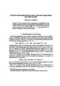
One may use DERIVE'Sgraphical capabilities to explore the quality of the given approximations by plotting both g and the calculated Taylor polynomials of g-l. We consider the last example. The function g(x) := xeX has a local minimum at x = -1 of value -e-' z -0.367879. It follows from complex analysis that the radius of convergence of the Thylor series of the inverse function does not exceed e - I . Thus only in the interval (-e-l,e-') can we expect that the Taylor polynomials converge to g-l(y). As an illustration Figure 1 shows the graph of g together with the first five Taylor polynomials TI,...,z of g-' that can be calculated by DERIVE simplifying VECTOR(INVERSE-TAYLOR(x*EXP(x),x, y, k), k, 1,s).

We mention that the calculation of Taylor polynomials for inverse functions is [6], where implemented in some Computer Algebra systems, e.g. in MATHEMATICA the function InverseTaylor[g-,x-, y-, nJ := InverseSeries[Series[g,(x,0, n)], y]

does the job desired. This method of inverting the Taylor polynomial of order n of g to get the Taylor polynomial of order n of g-', however, is static with respect to the order n. If we decide to calculate the Taylor polynomial of order n 1 later, we have to redo the whole calculation. With our method, in principle it is possible to work dynamically in the order as one may store the derivatives and limits up to order n that are already calculated in memory, i.e. one may work with streams and lazy evaluation.

+


We get for example

29


TAYLOR POLITOMIALS OF IMPLICIT F!JNCT!ONS

FIGURE 1. The graph of g ( x ) = xeX and the first 5 Taylor polynomials of g-I.

- - -- --.

-.-.

-r

r.

-.r

A"-,-"

*I

4. TAYLOR POLYNOMIAL SOLU I IONS ~r r ~ R Iavnvcn UIFFERENTIAL EQUATIONS

We consider the soiution of an initial value priiblcn; give:: 5.j an explicit first order differential equation y' = F ( x , y )

(3)

and initial data y(xo) = Yo.

Then-if the solution g ( x ) of (3)-(4) is n times differentiable-we search for its nth Taylor polynomial. A typical situation is an initial value problem (3)-(4) for a complex function g with analytic right hand side F. In this case the solution g is analytic in a neighborhood of the initial point xo (we hold on to use the symbol x rather than the usual z). To find its Taylor coefficients, we use the same method as before. Obviously

W. KOEPF


and with the derivatives list

an appiication of the aigoriiii~iifur iiiiplicit fiiii~iiiiiisjiieid~the Tqlnr polynoxia!. The DERIVEfunction DSOLVEl TAYLOR(f,x, y,xO,yO, nj := iiviPiiCii~i~fiOFi~A'di;(i,x, y , x O , yii, n, ~TERATES(DIF(S_, yjrf

t

i3ii-iy_,nj,d-,i,1-1

-

7))

uses this approach. We give ihe fdlowirig examples. DERIVE input

DERIVE output after

DSOLVEl_TAYLOR(y/x,x,y,xO, yo, 5)

'OX,

/ ww.r.t. x

x o

For the algorithmic construction of the Taylor series solution of homogeneous linear differentiai equations with poiynomiai coefficients (of arbii~ai-yorder) rather than Taylor polynomial approximations we again refer to [I]. We remark further that the same method can be applied to solve explicit first order systems, with the only difference that here d F k / a y then denotes the Jacobian.

TAYLOR POLYNOMIALS O F IMPLICiT FUNCTIONS

TAYLOR POLYNOMIAL SOLUTIONS OF HIGHER ORDER DIFFERENTIAL EQUATIONS


5.

In the case of an expiicit second order differentiai equation

the nth order Taylor polynomial of the solution of (5)-(6) has the form

>

and we can apply the same method as before after calculation of g'k)(xo) (k 2 ) . Let the given right hand side of ( 5 ) F ( x , y , u) he a function of the three varia'hies x , I., and v., that -n..mh A i C f e r e n t i ~ h l ~Again; we iterative!:, d i f f ~ r ~ n t jthe te ...-. is :Iftf.r: p-,Iu,,i. ,,iLL.Li,..,aeiL.

defining equatim of g X'!J.X) = F ( X , ~ ( X ) ? ~ ' ( X ) )

by the chain rule to get

and iteratively

To get g ( k ) ( ~(k~ )2 2 ) we have to evaluate g ( k ) ( x ) at the point x = xo, i.e. we take the limit for u -t yl, y -t yo, and x -t xo, which yields the result. This is done by the DERIVEfunction

DSOLVE2-TAYLOR(f, x, y, u, xO, YO,y l , n) : = DSOLVE2_TAYLORPUX(f,x, Y, u,xO, YO, Y 1 n. ITERATES(DIF(~-,u)*f + DIF(g_,y)*u + DIF(g-,x),g_,f, n - 2))

32

W. KOEPF


We present the following examples DERIVE input

DERIVE output after

DSOLVEZ-TAYLG~~EXP~ USIN ) ~jx),x,y, ~ ~ ~ i.i,O,O, 1,5)

-+ - - - + x . 12 120 6

ex4

x5

v]

x3

This method-as in the first order case-works independent of the linearity of the differeiitial ecjiiatioii. For the lincar differefitia! e q u d o n y J J ( x j+ p j x ) y l j x )

+ qjx));(xj = r ( x j

with initial conditions y(x0) = Yo

and y l ( x o ) = Y l

the DERIVEfunction

gives the Taylor polynomial solution of order n. The following are some examples DERIVE input

DERIVE output after

/Expand]

We remark that there is an obvious generalization of thc given technique to explicit differential equations of higher order (m E N)

with initial data


TAYLOR POLYNOMIALS O F IMPLICIT FUNCTIONS

References [ I ] W. Koepf, Power series in computer algebra, Journal of Symbolic Computation 13 (1992), 581-603. 12) W. Koepf, Algorithmic development of power series. In: Artificiai inieiiigeiicc and sy~~bc!ic mathmatical computing, ed. by J. Calmet and J. A. Campbell, International Conference AISMC-I, Karlsruhe, Germany, August 1992, Proceedings, Lecture Notes in Computer Science 737, Springer, BerlinHeilelberg, 1993, 195-213. [3] W. Kucpf, Examples [or the zlgorithmic calculation nf formal Puiseux. Laurent and power series, SIGSAM Bulletin 27 (1993). 20-32. [4] W. Koepf, A new algorithm for the development of algebraic functions in Puiseux series, Preprint B-92-21 Fachbereich Mathematik der Freien Universitat Berlin, 19%. [5] A. Rich, J. Rich and D. Stoutemyer, DERIVE User Manual, Version 2, Soft Warehouse, Inc., 3660 Waialae Avenue, Suite 304, Honolulu, HI, 96816-3236. [6] St. Wolfram, Mathematica. A system fur doing mathematics by Computer. Addison-Wesley Publ. Comp., Rcckood Cityj CA, 1991.