Instantaneous frequency estimation of polynomial ... - Semantic Scholar

2480

IEEE TRANSACTIONS ON SIGNAL PROCESSING, VOL. 47, NO. 9, SEPTEMBER 1999

Instantaneous Frequency Estimation of Polynomial FM Signals Using the Peak of the PWVD: Statistical Performance in the Presence of Additive Gaussian Noise Braham Barkat and Boualem Boashash, Fellow, IEEE

Abstract—The peak of the polynomial Wigner–Ville distribution (PWVD) has been recently proposed as an estimator of the instantaneous frequency (IF) for a monocomponent polynomial frequency modulated (FM) signal. In this paper, we evaluate the statistical performance of this estimator in the case of additive white Gaussian noise and provide an analytical expression for the variance. We show that for a given PWVD order, the estimator performance can be improved by a proper choice of the kernel coefficients in the PWVD. A performance comparison between the PWVD based IF estimator and another recently proposed one based on the high-order ambiguity function (HAF) is also provided. Simulation results show that for a signal-to-noise ratio larger than 3 dB, the proposed sixth-order PWVD outperforms the HAF in estimating the IF of a third- or fourth-order polynomial phase signal, evaluated at the central point of the observation interval. Index Terms—Estimation, instantaneous frequency, polynomial FM signals, polynomial Wigner–Ville distribution, statistical performance, time–frequency analysis, Wigner–Ville distribution.

I. INTRODUCTION

F

OR nonstationary signals, i.e., signals whose spectral contents vary with time, the frequency at a particular time is well described by the concept of instantaneous frequency (IF) [3], [4]. In many real-life applications such as radar, sonar, biomedical engineering, and automotive signals, the IF characterizes important physical parameters of the signals [8], [15]; therefore, it is desirable to have effective methods for IF estimation. The statistical performance of the IF estimator needs to be evaluated to provide the practitioner with a tool to judge the accuracy of the estimates. Time-frequency analysis was introduced as a tool to characterize the time-varying spectral contents of nonstationary signals. It is capable of displaying the temporal localization of the signal’s spectral components, i.e., it is very powerful in IF localization and estimation. The Wigner–Ville distribution (WVD), which is a member of a family of bilinear time–frequency distributions, was shown to be efficient in the estimation of a linearly frequency Manuscript received December 2, 1997; revised January 15, 1999. The associate editor coordinating the review of this paper and approving it for publication was Prof. Moeness Amin. The authors are with the Signal Processing Research Centre, School of Electrical and Electronics Systems Engineering, Queensland University of Technology, Brisbane, Australia (e-mail: [email protected]; [email protected]). Publisher Item Identifier S 1053-587X(99)06433-8.

modulated (FM) signal [14]. However, this property is no longer valid for nonlinear FM signals. For these types of signals, various higher order time–frequency distributions have been introduced. One of them is the polynomial Wigner–Ville distribution [6]. The peak of the polynomial Wigner–Ville distribution (PWVD) was proposed as an IF estimator for monocomponent polynomial FM signals [6]. The usefulness of the PWVD arises from its ability to localize energy along the IF law for such signals. That is, the PWVD represents higher order polynomial FM signals as delta functions in the time–frequency domain. In this paper, we evaluate the performance of the PWVD-based IF estimator in the case of additive white Gaussian noise. We demonstrate analytically that the estimator is unbiased and that its variance is a function of the kernel coefficients of the PWVD. We then illustrate how by an appropriate choice of these coefficients, we can design estimators with improved performance. An alternative technique was recently proposed in the literature to estimate the IF of a polynomial phase signal: the high-order ambiguity function (HAF) [12]. The principle of this parametric method is to nonlinearly transform the signal to obtain a sinusoid at a certain frequency that is directly related to the higher order coefficient of the phase of that signal [9]. A performance comparison between the PWVDbased IF estimator and the HAF-based IF estimator, for a polynomial phase signal in additive white Gaussian noise, is also presented. The paper is organized as follows. In Section II, a review of the PWVD is given. In Section III, we calculate the power of the crossterms in the PWVD. In Section IV, we derive the analytical expression for the estimator and compute its bias as well as its variance. Examples and simulation results are presented in Section V. Section VI gives a comparison between the PWVD method and the HAF method. The last section concludes the paper. II. THE POLYNOMIAL WIGNER–VILLE DISTRIBUTION The PWVD was designed to represent nonlinear polynomial FM signals of the form [6]

1053–587X/99$10.00  1999 IEEE

(1)

BARKAT AND BOASHASH: INSTANTANEOUS FREQUENCY ESTIMATION OF POLYNOMIAL FM SIGNALS USING THE PEAK OF THE PWVD

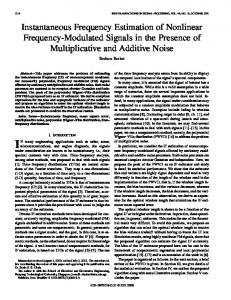
Fig. 1. WVD of a quadratic FM signal.

where the are real coefficients, and The IF of such a signal is a polynomial of order

2481

Fig. 2. Sixth-order PWVD of the same quadratic FM signal as in Fig. 1.

. , i.e., (2)

The PWVD was introduced in [6] as

III. POWER OF THE CROSS-TERMS IN THE PWVD In this section, we show that the noisy kernel of the PWVD can be written as the sum of two terms: the auto-terms and the cross-terms. We derive expressions of the auto-term and the cross-term power. These power expressions will be needed in subsequent derivations of the bias and the variance of the estimator in the next section. Consider the complex signal (4)

(3) where is an even integer that indicates the order of nonand ( linearity of the PWVD, and the coefficients ) are calculated so that the PWVD be real and optimal for representing polynomial FM signals given by (1) in the sense that it yields

is defined in (1), and is a zero-mean, complex where white Gaussian stationary noise with variance . The real and imaginary parts of the noise are assumed to be uncorrelated with equal variances. The kernel of the noisy signal is given by

(5) where is given by (2), and is Dirac’s delta function. . Note that the realness of the PWVD results in In addition, note that the WVD is a member of the class of , and . the PWVD’s with parameters ), a solution For the case of the sixth-order PWVD (i.e., , for the kernel coefficients gives [6] , and , yielding the sixth-order kernel

In the following, terms that contain one or more noise terms are called cross-terms (between noise and signal or between noise and noise), and the auto-terms refer to the noise-free terms. We can rewrite the previous expression as follows:

(6) is the number of the different coefficients , and , , is the multiplicity of each coefficient . Note , and [7]. that Each of the terms in the above product can be written as

where Fig. 1 shows the WVD of a quadratic FM signal. Fig. 2 of the same signal. The displays the PWVD of order time–frequency representation in Fig. 2 is characterized by the best achievable time–frequency resolution and the absence of artifacts. For this reason, it has been proposed as an IF estimator for polynomial FM signals. An efficient design procedure of PWVD’s has recently been proposed in [1].

(7)

2482


IV. VARIANCE AND THE INSTANTANEOUS

Therefore, the kernel of the noisy signal becomes

BIAS EXPRESSIONS FOR FREQUENCY ESTIMATOR

This section presents an evaluation of the statistical performance of the IF estimator using two different approaches. The first method is based on Taylor’s expansion, whereas the second method is based on the signal-to-noise ratio (SNR) of the PWVD kernel. We show that the two methods yield the same result. This result is a generalization of the results in [14] and [15]. A. Taylor’s Expansion Approach

(8) where the final terms indicated by dots are terms that involve products of more than one noise term. We note that the noisy kernel is the sum of two expressions. The first expression corresponds to the noise-free kernel, or auto-terms, whereas , corresponds to the the second expression, namely cross-terms. Assuming the power of the auto-terms is larger than the power of the discarded terms, we can write

The PWVD peak has been proposed as an IF estimator for polynomial phase signals. A performance analysis for showed that this polynomial phase signals up to order estimator provides an accurate means for IF estimation [5]. In this section, we generalize these results to the case of arbitraryorder polynomial phase signals embedded in white Gaussian noise. Assuming that there is no mismatch between the signal under consideration and the chosen PWVD, we evaluate the statistical performance of such an estimator. observations of the model in (4), and assuming a Given in the discrete-time rectangular window of length implementation of (3), the bias and the variance of the IF estimator, for high SNR, are found to be (13)

(14)

(9) Using the linearity of the expectation operator and the i.i.d. property of the complex Gaussian noise, it can be easily shown that the power of the cross-terms for a fixed nonzero lag is E For a zero lag

(10) , the cross-terms become

and the power in this case is (11) It is worth noting that (12) The above kernel conjugate symmetry property and the power expressions in (10) and (11) will be used extensively in the computations of the bias and the variance of the IF estimator in the following section.

Proof: Consider the discrete-time version of the noisy observations, in (4). It is assumed that the signal, given . sampling frequency is equal to unity

The kernel function of the PWVD attempts, at each time instant , to resolve a nonstationary signal into a sinusoid . Determining the IF is reduced to having frequency estimating the frequency of a discrete-time noisy sinusoid ) from the peak of the magnitude, or, equivalently, ( the squared magnitude, of the discrete-time Fourier transform of the kernel at each time instant . be the discrete-time Fourier transform of the Let . In the implementation of the discretenoisy kernel time Fourier transform in (3), the extent of the discrete-time to . In other words, we lag is taken from around the consider a rectangular window of length time instant in the evaluation of the discrete-time Fourier transform of the noisy kernel. The PWVD-based estimate of the true IF is defined as is maximum, the frequency at which the function i.e., (15)


To determine , consider the expansion of , i.e., to second order around

up

(16) Differentiating (16) with respect to

results in

(17) and using (15), we obtain

(18) Taking the expected value of (18), the expressions for the are found to be bias and variance in the estimate of

B. Signal-to-Noise Ratio Approach In [14], the authors showed that for high SNR, the variance of the IF estimator based on the peak of the WVD, i.e., the PWVD of order 2, reaches the Cramér–Rao lower bound for a linear FM signal. In this section, using the same procedure, we derive an expression for the asymptotic variance of the IF estimator based on the peak of the PWVD of an arbitrary order when applied to the appropriate nonlinear polynomial FM signal. The asymptotic variance of the discrete Fourier transformbased frequency estimate at high SNR and for a constant amplitude has been shown to be equal to [17] SNR

(19)

E (20) Evaluations of the expressions in the previous equations result in (13) and (14). The full derivations are given in Appendix A. Notes: The IF estimator variance is seen from (14) to decrease with large window length. Therefore, in the middle of odd) where the window length the time interval (assuming ), can be chosen equal to the signal length (i.e., the variance is minimum and is found to be equal to

(22)

, stands where SNR, which is given by SNR for the signal-to-noise ratio (SNR) in the discrete Fourier , which is the number of transform (DFT) scaled by represents the independent signal samples. The quantity represents the power of the power of the sinusoid, and noise. For convenience and as a matter of comparison with . Then, the above our previous results, we let equation becomes SNR

E

2483

(23)

Based on this result, and in order to determine the variance of the PWVD peak-based IF estimator, we must first determine the SNR in the DFT of the kernel in the PWVD at each time instant . Using (8), we see that at each time instant , the noisy kernel embedded in white Gaussian reduces to a sinusoid . In our case, the power of the sinusoid is equal to noise , whereas, the power of the cross-terms, or noise, is given (here, it is assumed, for simplicity, by is equal to the power at that the power at time-lag ; refer to Section III). However, due other time-lags to the kernel conjugate symmetry [see (12)], the number of ) but only independent samples in the noise is not ( . Therefore, the SNR in the DFT of the PWVD kernel . Replacing these expressions in (23), is scaled by we find

(21) At other time instants , the implementation of the PWVD necessitates smaller window lengths, resulting in a decrease in the statistical performance of the IF estimator. We also observe that the variance is a function of the kernel coefficients of the PWVD. Thus, a proper choice of these coefficients will improve the performance of the estimator. For example, for the sixth-order kernel given in Section II, ; if we choose the coefficients to be we have . This represents a 40% different, we can obtain decrease in the variance. This point will be discussed in more detail in Section V.

(24) sufficiently large and approximating Assuming by , we obtain the expression of the variance in (14). Note—Second-Order PWVD: The PWVD of order two reduces to the WVD. It can be implemented in two different ways, using either (25)

2484


It can be shown [15] that for a PWVD, this threshold can be approximated by

or equivalently

(26)

[dB]

For the first method, there is an inherent frequency scaling by a factor of two. This means that the frequency estimate obtained from the peak of the WVD must be corrected by the same factor. This implies that the IF estimator variance must be reduced by four [14], that is, (14) becomes For a fixed window length ( ), the threshold for the PWVD of order six is approximately 7 dB higher than that of the WVD.

This result can also be obtained by direct calculation as we did for the general case, but this time, we have a factor four in the exponential in (25). At the middle of the time interval, the window length ) can be chosen equal to the signal length . In this ( case, we obtain the same result as the one in [14], namely,

V. RESULTS

AND

DISCUSSIONS

In this section, several experiments are conducted on both a linear FM signal and then a quadratic FM signal, and the results are discussed. However, using the appropriate PWVD’s, higher order polynomial FM signals can also be considered. A. Linear FM Case

(27)

We should emphasize here that this result is valid only at the middle of the signal duration and is not valid at other times as suggested in [14] and [15]. For the second method of implementation of the WVD, the signal is first interpolated (by a factor of 2), and then, at each time , the DFT of the kernel is computed. In this method, there is no frequency scaling. At the middle of the time interval, for a window length equal to the signal length, the IF estimator variance is found to be

(28)

In this case, the variance is larger than the variance obtained for the WVD in the first method. More details are given in Section V. C. Threshold of the Variance The derivation of the variance of the PWVD-based IF estimator was obtained under the assumption that the SNR is high. For a fixed window length and decreasing SNR or for fixed SNR and decreasing window length, the estimator variance reaches a threshold beyond which the variance increases dramatically.

The signal under consideration is a unit-modulus linear FM and a sampling frequency equal to signal of length one. We add a complex white Gaussian noise to the signal . The frequency of and define the SNR as SNR the peak of the PWVD, at the middle point of the signal interval, is chosen as an estimate of the frequency at that time instant. The window length is taken equal to the signal length ), except where it is stated otherwise. Monte ( Carlo simulations for 1000 realizations are run for each SNR. 1) The WVD Case: As stated earlier, there are two methods in implementing the WVD, and the IF estimator variance depends on the method applied. For the first method, we use the WVD expressed by (25). In other words, there is no interpolation of the analytic signal in the time–frequency computation. In this case, the theoretical variance is given by (27). In Fig. 3, we plot the simulation results, represented by “ ,” for the IF estimator variance as a function of the SNR (expressed in decibels). The dotted line represents the theoretical variance for this case, namely (27). The Cramér–Rao bound for a linear FM signal [11], at the middle of the signal duration, is represented by the dashed line. As expected, and in agreement with the results in [14], the IF estimator is efficient for that particular time instant. For the second method, we compute the WVD using (26). In this case, an interpolation of order two of the analytic signal is necessary in order to obtain the signal samples at noninteger values of time. The simulation results are plotted in Fig. 4, where the IF estimator variance is represented by “ ,” and the theoretical variance, in this case given by (28), is represented by the dotted line. We observe here that our estimator is not efficient.


Fig. 3. Peak of the WVD with no interpolation is used as an IF estimator, at the middle of the observation interval, for a linear FM signal in additive white Gaussian noise. The window length is equal to the signal length ). (2

2485

Fig. 5. Plots of Figs. 4 and 5 are combined here for a closer comparison.

M + 1 = N = 129

Fig. 6. Peak of the new sixth-order PWVD is used as an IF estimator at the middle of observation interval for a linear FM signal in additive white Gaussian noise. Two different window lengths are considered. Fig. 4. Peak of the WVD with interpolation is used as an IF estimator at middle of observation interval for a linear FM signal in additive white Gaussian noise. The window length is equal to the signal length ( ).

2M +1 = N = 129

Based on these results, we conclude that the estimated variances of the IF for a linear FM signal, at the middle of the time interval, are in accordance with the theoretical variances derived earlier. In Fig. 5, we combine the results of Figs. 3 and 4 for a better comparison. In particular, note that as expected, the IF estimator variance is smaller when the peak of the WVD is used without interpolation. 2) Higher Order PWVD’s Case: We limit ourselves to the sixth-order PWVD. In Section II, we presented one kernel for the sixth-order PWVD, which we rewrite here for convenience as (29) Theoretically, there is an infinite number of solutions to the sixth-order PWVD kernel coefficients. In [2], we computed the optimum set of coefficients. This optimality assures the minimum order of interpolation of the signal in the implementation of the distribution as well as the minimum variance of the IF estimator when the peak of the PWVD is used as an estimator. The optimal kernel has all its coefficients different from . This means that the variance one another; then,

of the IF estimator is lowered by 40% compared with the variance when the above kernel, which is referred to as the old kernel, is used in IF estimation. This reduction represents a difference of about 2.2 dB in the IF estimator variances. The optimal kernel is given by [2]

(30) Simulation results showed that the IF estimator variance based on the old PWVD and the IF estimator variance based on the optimal, referred to as new, sixth-order PWVD, are identical except for the 2-dB difference. Therefore, to avoid redundancy, we display only the results of the new PWVD. In Fig. 6, we plot the IF estimator variances for two different window lengths. The “ ” correspond to the longer window ), whereas the “ ” correspond to the smaller ( ). Note how the variance with the window ( smaller window length is higher than the variance with the larger one. This is in accordance with the derived theoretical results in (14). The threshold variance of the sixth-order PWVD, either old or new, is higher than that of the WVD. For a fixed window length, the theoretical difference approximates 7 dB for the old

2486


be a polynomial phase discrete time signal. The signal model can, therefore, be written as

The signal can be rewritten in the form

where is also white and Gaussian. The kernel of the discrete-time noisy signal, using (5), is

Fig. 7. Peak of the new PWVD is used as an IF estimator at the middle of observation interval for a quadratic FM signal in additive white Gaussian ). noise. The window length is equal to the signal length (2

M +1 = N = 129

The expressions above allow us to rewrite the noisy kernel as

PWVD and it is about 4 dB for the new PWVD. This result is also confirmed by the simulations. B. Quadratic FM Case We consider a quadratic FM signal under the same conditions as in the previous case. As the WVD is inappropriate for a nonlinear FM signal, we consider, in this case, the IF estimation using the peak of the new sixth-order PWVD. Fig. 7 displays the IF estimator variance at the middle of the signal interval. The Cramér–Rao of a quadratic FM signal [11] is plotted for comparison. To conclude this section, we can say that the results of the Monte Carlo simulations for both the WVD and the PWVD of order six confirm our theoretical derivations.

(31) with

being the IF at time instant is given by

, and the quantity

VI. COMPARISON OF THE PWVD WITH HIGH-ORDER AMBIGUITY FUNCTION

THE

The high-order ambiguity function (HAF) algorithm is a parametric method that has also been proposed for IF estimation of polynomial FM signals [12]. The asymptotic variances of the estimates were shown to be close to the Cramér–Rao bound (CRB) for high SNR [13]. In this section, we compare the statistical performances of the PWVD-based IF estimator with the HAF-based IF estimator in estimating the instantaneous frequency of a polynomial FM signal. In particular, we show that the new sixthorder PWVD (see previous section) outperforms the HAF in estimating the IF of a quadratic, or a cubic, FM signal in additive white Gaussian noise at the central point of the observation interval. A. Derivations Both the PWVD and the HAF algorithms search for the maximum point of a discrete Fourier transform at every fixed time instant . The perturbation of the measured maximum point from the real one is the error under consideration. Let the additive interference be complex circular white Gaussian and the unit-modulus signal with variance equal to

If we let be the point of local maximum of the discrete nearest to Fourier transform of the noisy sinusoid and based on the derivation in [13], we obtain the true IF

(32)

and being the number of with in the PWVD kernel. the coefficients Full details of the derivation are given in Appendix B. B. Example and Comparisons Consider the estimation of the IF at the middle of the time interval of a unit-modulus quadratic FM signal. The and its sampling signal length is assumed equal to frequency equal to 1. If the old sixth-order PWVD is used in


2487

noise. An analytical expression for the variance has been derived. We have shown that the estimator is unbiased, and its variance is a function of the kernel coefficients. This variance can be reduced by a proper choice of these coefficients. A performance comparison of the PWVD and the HAF-based IF estimators showed that the new sixth-order PWVD outperforms the HAF in estimating the IF of a thirdor fourth-order polynomial phase signal at the central point of the observation interval for a signal to noise ratio larger than 3 dB. APPENDIX A

Fig. 8. IF variances for the old sixth-order PWVD (dashed line), the new PWVD (continuous line), and the HAF (dot-dashed line). The Cramér–Rao bound is represented by the dotted line. The window length is equal to the ). signal length (2

This Appendix provides the derivation of the bias and the variance of the IF estimator when using the peak of the PWVD in the case of white Gaussian noise. The discrete time version of the noisy kernel in (8), for a time instant and a lag , is given by

the estimation, then the corresponding IF estimator variance is found to be

Thus

M + 1 = N = 129

with However, if the new sixth-order PWVD is used, then

The error based on the HAF is well detailed in [13]. In Fig. 8, we plotted the above variances as well as the HAF-based IF estimator variance versus the SNR in decibels. Note the superiority of the new sixth-order PWVD over the two other estimators. For a cubic FM signal, the results were similar. We should observe, as stated in previous sections, that the statistical performance of the PWVD-based IF estimator degrades as we move away from the middle point of the time interval. Apart from the signal interpolation that is done only once in the PWVD interpolation, we note that for IF estimation, and at a fixed time instant, the PWVD requires only one onedimensional (1-D) search for the maximum of the discrete time Fourier transform of the kernel. However, the HAF requires a multiple (equal to the order of the polynomial phase signal) 1D search to estimate all the coefficients and then the IF. Thus, at a fixed time instant, the HAF is computationally more complex. On the other hand, the PWVD becomes computationally more complex if the number of time instants where the IF is to be estimated is larger than the order of the polynomial phase signal under consideration. VII. CONCLUSIONS The performance of IF estimators using the peak of the polynomial Wigner–Ville distribution is evaluated for the case of polynomial FM signals in additive white Gaussian

The squared magnitude of the above discrete Fourier transform of the noisy kernel can be written as follows:

Re (33) Assuming that for high SNR, we can write

Recalling that

, which is valid

[7] and using

2488


the denominator in (19) and (20) evaluated at to be

is found

The expected value of each term in the above equation is found to be E

Therefore, the expressions for the bias and variance can now be written as E

E

(34) E

E

(35)

in (33) by the first two Now, we approximate terms on the right-hand side and derive with respect to

where is the cross-terms power derived in Section III. Inserting these results in (35) and simplifying, we obtain for the variance

APPENDIX B Re (36)

This Appendix outlines the derivation details of the result given in Section VI. The perturbation error is given by [13]

Using the i.i.d. property of the noise and the linearity of the expectation operator, the expected value of the precedent is found to be equal to zero. expression evaluated at From (34), we have

Re

Re

For the variance, we need to evaluate (36) at take the square of the result to obtain

Im

and

under the assumptions .

A1) A2)

.

is the Fourier transform of the discrete random , and is its th derivative. additive interference and Im stand for real and imaginary parts of the Re means that all the expression. The notation are uniformly bounded in , whereas the moments of means that . notation for all [using (39) It should be noted that E and (40) below]. This means that the estimator is unbiased, as expected. In our case, the above assumptions hold, and the asymptotic variance of the error is found to be [16]

E

(37)


Let us now evaluate the expectation in the above equation.

2489

Following the same procedure, we can show that E

E

(42)

, we have , and For . Taking this into E consideration and inserting the above expressions in (37), we obtain

E

E E

E which reduces to (32). E APPENDIX C E (38) In order to evaluate the precedent expression, the following formulae are used [13]: E

E

(39)

On request by a reviewer, the authors have included a brief comparison between the PWVD and the HAF for the estimation of the IF in the case of time-varying amplitude monocomponent polynomial FM signal. In [10], the authors show that the discrete-time HAF, then called DPT, for a time-varying amplitude signal [ is a polynomial of , and is a real function of ] is equal to the convolution, in frequency, with the HAF of , i.e., of the HAF of DPT

(40)

E

, and let be the multiplicity of coefficient Let . Grouping all the kernel terms having the same coefficient together and using (40), the first term of (38) becomes E

with , and is the number of the different coefficients of the terms in the PWVD kernel. The second term of (38) gives us exactly the same result as the first term. The third and the fourth terms of (38) are found as well as equal to unity by using the i.i.d. property of (39). Therefore, we obtain

DPT Thus, for each the polynomial

DPT , assuming the order of known, the above equation becomes

DPT DPT where , is the coefficient under consideration, and is the sampling frequency. In the above, is more correct a Sinc function whose maximum is at than a delta function, but this will not affect the following discussion. In general, the maximum of the above expression is not guaranteed to be at , even for the noiseless signal, and . Only is highly dependent on the HAF of the amplitude is symmetrical about the zero axis with its if the HAF of maximum at frequency zero can we recover the coefficient (for example, in the case of slowly varying real amplitude). Otherwise, the HAF of the time-varying amplitude signal cannot give us the correct coefficients of the polynomial. On the other hand, for a PWVD, we have

E Thus, for every time instant , we have (41)

FT

2490


where is the IF at that particular time expression is

. The other

FT with being a constant equal to the product of all ampliselected in the window tudes of the samples of to . Therefore, at high SNR, the PWVD of the timealways has its maximum at varying amplitude signal . We see that from the IF estimation point of view, the PWVD has always its maximum at the IF; however, the HAF, in general, does not guarantee this. For this, at high SNR, we expect the PWVD to be more appropriate for IF estimation for a time-varying amplitude polynomial FM signal. Note that for both algorithms, the resolution, as well as the effective SNR, are decreased. This means that in the time-varying amplitude case, the statistical performance of the above estimators is less than that of a constant amplitude signal. ACKNOWLEDGMENT The authors would like to thank Prof. A. M. Zoubir and Dr. B. Ristic for their useful suggestions and comments. REFERENCES [1] B. Barkat and B. Boashash, “Design of higher-order polynomial Wigner–Ville distributions,” IEEE Trans. Signal Processing, this issue, pp. 2608–2611. [2] B. Barkat, “Note on the coefficients precision and selection in the implementation of the PWVD,” in Proc. 2nd Workshop on Signal Processing Applications, Brisbane, Australia, Dec. 4–5, 1997, pp. 131–134. [3] B. Boashash, “Interpreting and estimating the instantaneous frequency of a signal—Part I: Fundamentals,” Proc. IEEE, vol. 80, pp. 520–538, Apr. 1992. [4] , “Interpreting and estimating the instantaneous frequency of a signal—Part II: Algorithms,” Proc. IEEE, vol. 80, pp. 539–569, Apr. 1992. [5] , “Time-frequency signal analysis: Past, present and future trends,” in Control and Dynamic Systems, C. T. Leonides, Ed. New York: Academic, 1996, vol. 78, Digital Control and Signal Processing Systems and Techniques, ch. 1, pp. 1–71. [6] B. Boashash and P. J. O’Shea, “Polynomial Wigner–Ville distributions and their relationship to time-varying higher order spectra,” IEEE Trans. Signal Processing, vol. 42, pp. 216–220, 1994. [7] B. Boashash and B. Ristic, “A time-frequency perspective of higherorder spectra as a tool for nonstationary signal analysis,” in HigherOrder Statistical Signal Processing, B. Boashash, E. J. Powers, and A. M. Zoubir, Eds. London, U.K.: Longman, 1995, ch. 4. [8] D. König and J. F. Böhme, “Wigner–Ville spectral analysis of automative signals captured at knock,” Appl. Signal Process., vol. 3, pp. 54–64, 1996. [9] A. Ouldali and M. Benidir, “Distinction between polynomial phase signals with constant amplitude and random amplitude,” in Proc. IEEE Int. Conf. Acoust., Speech, Signal Process., Munich, Germany, Apr. 21–24, 1997, vol. 5, pp. 3653–3656. [10] S. Peleg and B. Friedlander, “The discrete polynomial-phase transform,” IEEE Trans. Signal Processing, vol. 43, pp. 1901–1915, Aug. 1995. [11] S. Peleg, B. Porat, and B. Friedlander, “The achievable accuracy in estimating the instantaneous phase and frequency of a constant amplitude signal,” IEEE Trans. Signal Processing, vol. 41, pp. 2216–2223, June 1993.

[12] B. Porat, Digital Processing of Random Signals. Englewood Cliffs, NJ: Prentice-Hall, 1994. [13] B. Porat and B. Friedlander, “Asymptotic statistical analysis of the highorder ambiguity function for parameter estimation of the polynomialphase signal,” IEEE Trans. Inform. Theory, vol. 42, pp. 995–1001, May 1996. [14] P. Rao and F. J. Taylor, “Estimation of IF using the discrete Wigner–Ville distribution,” Electron. Lett., vol. 26, pp. 246–248, 1990. [15] D. C. Reid, A. M. Zoubir, and B. Boashash, “Aircraft flight parameter estimation based on passive acoustic techniques using the polynomial Wigner–Ville distribution,” J. Acoust. Soc. Amer., vol. 102, no. 1, pp. 207–223, 1997. [16] G. Reina and B. Porat, “Comparative performance analysis of two algorithms for IF estimation,” in Proc. 8th IEEE Signal Process. Workshop Stat. Signal Array Process., Corfu, Greece, June 1996, pp. 448–451. [17] D. C. Rife and R. R. Boorstyn, “Single tone parameter estimation from discrete-time observations,” IEEE Trans. Inform. Theory, vol. IT-20, pp. 591–598, 1974.

Braham Barkat was born in Algiers, Algeria, in 1961. He joined the National Polytechnic Institute of Algiers (ENPA) in 1980 and received the degree of “Ingenieur d’Etat” in electronics in 1985. In 1986, he joined the University of Colorado, Boulder, where he received the M.S. degree in control systems in 1988. In 1989, he joined the University of Blida, Blida, Algeria, where he held the position of Lecturer in digital and advanced control systems. In 1996, he joined the Signal Processing Research Center, Queensland University of Technology, Brisbane, Australia, as a Senior Research Assistant and then as a Ph.D. student in signal processing. He expects to graduate in 1999. His research interests include time–frequency signal analysis, estimation and detection, statistical array processing, and embedded control and digital signal processing systems. Mr. Barkat received the “Best Student Award” in 1980 for the highest point average on the Baccalaureate Exam in Algeria.

Boualem Boashash (SM’89–F’99) received the Diplome d’ingenieur-Physique-Electronique from the ICIP University of Lyon, Lyon, France, in 1978, the M.S. degree from the Institut National Polytechnique de Grenoble (INPG), Grenoble, France, in 1979, and the Doctorate (DocteurIngenieur) degree from INPG in May 1982. In 1979, he joined Elf-Aquitaine Geophysical Research Center, Pau, France. In May 1982, he joined the Institut National de Sciences Appliqées de Lyon. In 1984, he joined the Electrical Engineering Department, University of Queensland, Brisbane, Australia, as a Lecturer. He was appointed Senior Lecturer in 1986 and Reader in 1989. In 1990, he joined the Graduate School of Science and Technology, Bond University, Gold Coast, Australia, as a Professor of Electronics. In 1991, he joined the Queensland University of Technology, Brisbane, as the Foundation Professor of Signal Processing and Director of the Signal Processing Research Center. He is the editor of two books, has written more than 200 technical publications, and has supervised more than 20 Ph.D. students and five M.S. students. His research interests are time–frequency signal analysis, spectral estimation, signal detection and classification, and higher order spectra. He is also interested in wider issues such as the effect of engineering developments on society. Prof. Boashash was Technical Chairman of ICASSP 1994: the premium conference in signal processing. He is a Fellow of IE Australia and of the IREE.