riences similar to the popular bullet-time sequence. We believe that this type of application will greatly enhance shared human experiences spanning from ...
CrowdCam: Instantaneous Navigation of Crowd Images using Angled Graph Aydın Arpa1 Luca Ballan2 Rahul Sukthankar3 Gabriel Taubin4 Marc Pollefeys2 Ramesh Raskar1 1
MIT, 2 ETH Zurich, 3 CMU, 4 Brown University
Abstract
In this paper, we describe a solution to this problem by providing the user with the possibility of using his/her cellphone or tablet to navigate specific salient moments of an event right after they happened, generating bullet time experiences of these moments, or interactive visual tours. To do so, we exploit the known fact that, important moments of an event are densely photographed by its audience using mobile devices. All of these photos are collected on a centralized server, which sorts them spatiotemporally, and sends back results for a pleasant navigation on mobile devices. (see Figure 1)
We present a near real-time algorithm for interactively exploring a collectively captured moment without explicit 3D reconstruction. Our system favors immediacy and local coherency to global consistency. It is common to represent photos as vertices of a weighted graph, where edge weights measure similarity or distance between pairs of photos. We introduce Angled Graphs as a new data structure to organize collections of photos in a way that enables the construction of visually smooth paths. Weighted angled graphs extend weighted graphs with angles and angle weights which penalize turning along paths. As a result, locally straight paths can be computed by specifying a photo and a direction. The weighted angled graphs of photos used in this paper can be regarded as the result of discretizing the Riemannian geometry of the high dimensional manifold of all possible photos. Ultimately, our system enables everyday people to take advantage of each others’ perspectives in order to create on-the-spot spatiotemporal visual experiences similar to the popular bullet-time sequence. We believe that this type of application will greatly enhance shared human experiences spanning from events as personal as parents watching their children’s football game to highly publicized red carpet galas.
To promote immediacy, and interactivity, our system needs to provide a robust, lightweight solution to the organization of all the visual data collected at a specific moment in time. Today’s tools that address spatiotemporal organization mostly starts with a Structure From Motion (SFM) operation [13], and largely assumes accurate camera poses. However this assumption becomes an overkill when immediacy and experience is more important than the accuracy on these estimations. Furthermore, SFM is a computationally heavy operation, and does not work in a number of scenarios including non-Lambertian environments. Our solution instead focuses on immediacy and local coherency, as opposed to the global consistency provided by full 3D reconstruction. We propose to exploit sparse feature flows in-between neighbouring images, and create graphs of photos using distances and angles. Specifically, we build Weighted Angled Graphs on these images, where edge weights describe similarity between pairs of images, and angle weights penalize turning on angles while traversing paths in the subjacent graph. In scenarios where the number of images is large, computational complexity of finding neighbours is reduced by employing visual dictionaries. If the event of interest has a focal object, we let the users enter this region of interest via simple gestures. Afterwards, we propagate features from user provided regions to all nodes in the graph, and stabilize all flows that has the target object. In order to globally calculate optimum smoothest paths, we project our graph to a dual space where triplets become pairs, and angle costs are projected to edge costs and therefore can simply be calculated via short-
1. Introduction All of us like going to public events to see our favourite stars in action, our favourite sports team playing or our beloved singer performing. Attending these events in first person at the stadium, or at the concert venue, provides a great experience which is not comparable to watching the same event on television. While television typically provides the best viewpoint available to see each moment of the event (decided by a director), when experiencing the event in first person at the stadium, the viewpoint of the observer is restricted to the seat assigned by the ticket, or his/her visibility is constrained by the crowds gathered all around the performer, trying to get a better view of the event. 1
...
(a)
(b)
(c)
Figure 1. Imagine you are at a concert or sports event and, along with the rest of the crowd, you are taking photos (a). Thanks to other spectators, you potentially have all possible perspectives available to you via your smart phone (b). Now, almost instantly, you have access to a very unique spatiotemporal experience (c).
est path algorithms.
1.1. Contributions In this paper, our contributions are as follows: • Novel way to collaboratively capture and interactively generate spatiotemporal experiences of events using mobile devices • Novel way to organize captured images on an Angled Graph by exploiting the intrinsic Riemannian structure • A way to compute the geodesics and the globally smoothest paths in an angled graph • An optional object based view stabilization via collaborative segmentation
2. Related Work Large Collections of Images: There is an ever-increasing number of images on the internet, as well as research pursuing storage [6] and uses for these images. However, in contrast with exploring online collections, we focus on transient events where the images are shared in time and space. Photo Tourism [22] uses online image collections in combination with structure from motion and planar proxies to generate an intuitively and browsable image collection. We instead do not aim at reconstructing any structure, shape, or geometry of the scene. All the processing is image based. [21, 20, 18] achieved smooth navigation between distant images by extracting paths through the camera poses estimated on the scene. Similar techniques were used to create tourist maps [9], photo tours [13], and interactive exploration of videos [2, 24]. Along with the same line of research, we also present, in this paper, how to navigate between the images. In contrast to prior work however, we do not require expensive pre-processing steps for scene reconstruction. The relationship between images is calculated in near-real time. Other works using large image collections to solve computer vision problems include scene recognition [19, 25] and image completion [11].
Computing Shortest Paths: Finding the shortest path between two points in a continuous curved space is a global problem which can be solved by writing the equation for the length of a parameterized curve over a fixed one dimensional interval, and then minimizing this length using the calculus of variations. Computing a shortest path connecting two different vertices of a weighted graph is a well studied problem in graph theory which can be regarded as the discrete analog of this global continuous optimization problem. A shortest path is a path between the two given vertices such that the sum of of the weights of its constituent edges is minimized. In a finite graph a shortest path always exists, but it may not be unique. A classical example is finding the quickest way to get from one location to another on a road map, where the vertices represent locations, and the edges represent segments of roads weighted by the time needed to travel them. Many algorithms have been proposed to find shortest paths. The best known algorithms for solving this problem are: Dijkstra’s algorithm [7], which solves the single-pair, single-source, and single-destination shortest path problems; the A? search algorithm [10], which solves for single pair shortest path using heuristics to try to speed up the search; Floyd-Warshall algorithm [8], which solves for all pairs shortest paths; and Johnson’s algorithm [12], which solves all pairs shortest paths, and may be faster than Floyd-Warshall on sparse graphs.
Organizing Images: Existing techniques use similaritybased methods to cluster digital photos by time and image content [4], or other available image metadata [26, 16]. For image based matching, several features have been proposed in literature, namely, KLT [23], SIFT [14], GIST [17] and SURF [3]. Each of these features have its own advantages and disadvantages with respect to speed and robustness. In our method, we propose to use SIFT features, extracted from each tile of the image, and to individually quantized them using a codebook in order to generate a bag-of-words representation [5].
Figure 2. A set of input images (I) are converted to a set of SIFT features (F). In case of a large number of the images, a visual dictionary (D) is employed to represent every image via a high dimensional vector (C). Nearest Neighbours (NN) are found for each image, and sparse feature flow (FF) vectors are extracted. If there is a object of interest, and few users have manually entered its region, this input is used to stabilize (S) the views. A graph (G) is generated where nodes are images and edges represent distances. In this graph, angles are present but only on triplets. The graph (G) is then projected to a dual graph (G*), where edges have both distance and angle costs. Then given the desired Navigation (N) mode from user, the system creates the smoothest path (P), and generates a rendering (R).
3. Algorithm Overview Our approach starts with users taking photos on their mobile devices using our web-app. As soon these photos are taken, they are uploaded to a central server along with metadata consisting of time and location, if available. Afterwards, applying a coarse spatiotemporal filtering using this metadata provides us the initial ”event” cluster to work on. Event clusters are sets of images taken at similar time and location (Section 4). Sparse feature flows within neighbouring images are then estimated. For large event clusters, computational complexity of calculating feature flow for each pair of images is drastically reduced by employing visual dictionaries (Section 4.1). The computed feature flows are then used to build a Weighted Angled Graph on these images (Section 5). Each acquired image is represented as a node in this graph. Edge weights describe similarity or distance between pairs of photos, and angle weights penalize turning on angles while traversing paths in the subjacent graph. Once a user swipes his finger towards a direction, the system computes the smoothest path in that direction and starts the navigation. This results in a bullet time experience of the captured moment. Alternatively user can pick a destination photo, and the system finds the smoothest path in between. The algorithm ensures that the generated paths lie on a geodesic of the Riemannian manifold of the collected images. This geodesic is uniquely identified by the initial photo (taken by the user) and the finger swiping direction. To this end, Section 5.2 introduces the novel concept of straightness and of minimal curvature in this space (Section 5.4), and propose an efficient algorithm to solve for it. In particular, to simplify the calculations and to ensure near realtime performances, in finding the globally optimum smoothest path, we project our graph to a dual space
where triplets become pairs, and angle costs are projected to edge costs. Then Dijkstra’s shortest path algorithm is applied to give us globally optimum smoothest path. For each event cluster, if there is a focal object of interest, the user can enter the object’s region via a touch gesture. Our algorithm propagates the features from user provided regions to all the nodes in the graph, and stabilize all the flows related to the target object. Figure 2 shows an overview of the proposed pipeline.
4. Coarse Spatiotemporal Sorting Photos are uploaded continuously to the server, as soon as they are taken. The server performs an initial clustering of these images based on the location and time information stored in the image metadata. Depending on the event, and the type of desired experience, users can interactively select the spatiotemporal window within which to perform the navigation. For instance, for a concert and a sports event, users might prefer large spatial windows whereas, for a street performance, small spatial windows are preferred. Concerning the time dimension, this can go between 1 or 2 seconds for very fast events, to 10 seconds in case of almost static scenarios or very slow events, like an orchestra performance. In terms of temporal resolution, cellphone time is quite accurate thanks to indirect syncing of its internal clock to the atomic clocks installed in satellites and elsewhere. However, spatial information provided by sensors needs extra care as it is too coarse to be used in smooth visual navigation. Its accuracy drastically decreases in case of indoor events. In order to attain better spatial resolution, we exploit sparse feature flows in between neighbouring photos, as described in the following sections.
4.1. Efficiently Finding Neighbours with Visual Dictionaries Naively, the computational complexity of calculating the feature flow for each pair of images would be O(N 2 ), and therefore posits infeasible when the number N of photos in the cluster is large. In these cases, we reduce the computational complexity by employing a visual dictionary [5], and near-neighbor search algorithms [15]. By doing this, we reduce the complexity to O(KN ) where K is the number of neighbours. Dictionaries can be catered for specific venues, or specific events. They can be created on the fly, or can be reutilized per location. For instance, in a fixed environment like a basketball stadium, it is really advisable to create a dictionary for the environment beforehand and cache it for that specific location. For places where the environment is unknown, and the number of participants is large, it is advisable that a dictionary is created on the fly at the very beginning of the event, and shared by all. For the samples we used, our rule of thumb was that we employed a dictionary if the number of photos were more than 50.
5. Weighted Angled Graph In mathematics a geodesic is a generalization of the notion of a straight line to curved spaces. In the presence of a Riemannian metric, geodesics are defined to be locally the shortest path between points in the space. In Riemannian geometry geodesics are not the same as shortest curves between two points, though the two concepts are closely related. The main difference is that geodesics are only locally the shortest path between points. The local existence and uniqueness theorem for geodesics states that geodesics on a smooth manifold with an affine connection exist, and are unique. More precisely, but in simple terms, for any point p in a Riemannian manifold, and for every direction vector ~v away from p (~v is a tangent vector to the manifold at p) there exists a unique geodesic that passes through p in the direction of ~v . A weighted graph can be regarded as a discrete sampling of a Riemannian space. The vertices correspond to point samples in the Riemannian space, and the edge weights to some of the pairwise distances between samples. However, this discretization neither allows us to define a discrete analog of the local geodesics with directional control, nor the notion of straight line. Given two vertices of the graph connected by an edge, we would like to construct the straightest path, i.e. the one that starts with the given two vertices in the given order, and continues in the same direction with minimal turning. To define a notion of straight path in a graph we augment a weighted graph with angles and angle weights. An angle of a graph is a pair of edges with a common vertex, i.e., a
Figure 3. The angled graph is converted to a weighted graph in order to simplify the computation of the global shortest path.
path of length 2. Angle weights are non-negative numbers which penalizes turning along the corresponding angle. Graph angles are related to the intuitive notion of angle between two vectors defined by an inner product. This definition extends the relation between edges and edge weights in a natural way to angles and angle weights. In a Riemannian space, using the inner product derived from the Riemannian metric, the angle α between two local geodesics passing through a point p with directions defined by tangent vectors ~v and w ~ is well defined. In fact, the cosine of the angle (0 ≤ α ≤ π) is defined by the expression cos(α) =
h~v , wi ~ , k~v k kwk ~
(1)
where h~v , wi ~ is the inner product of ~v and w ~ in the metric, and k~v k denotes the length (L2 norm) of the vector ~v . Within this context, angle weights can be defined as a nonnegative function s(α) ≥ 0 defined on the angles. A graph G = (V, E) comprises a finite set of vertices V , and a finite set E of vertex pairs (i, j) called edges. A weighted graph G = (V, E, D) is a graph with edge weights D, an additional mapping D : E → R which assigns an edge weight dij ≥ 0 to each edge (i, j) ∈ E. An Angled Graph G = (V, E, A) is a graph augmented with a set of angles A. Given a path (i, j, k), an angle is defined as the high dimensional rotation between edges (i, j) and (j, k). Finally, a Weighted Angled Graph G = (V, E, D, A, S) is an weighted graph augmented with a set of angles A and and angle weights S, a mapping S : A → R which assigns an angle weight sijk ≥ 0 to each angle (i, j, k) ∈ A. Since edges (j, i) and (j, i) are considered identical, angles (i, j, k) and (k, j, i) are considered identical as well.
5.1. Angles as Navigation Parameters We are more interested in minimizing the path energy one step at a time, i.e. within the neighborhood of each vertex: if (i, j) is an edge, the vertex k in the first order neighborhood of j which makes the path (i, j, k) straightest is
the one that minimizes sijk . The local straightest path is the path with the lowest energy to the next node with respect to edge and angle weights. This energy is written as a linear combination of both measurements: λ dij + (1 − λ) skij
B
A
AB
C
BC
(2)
Where node k is the previous node in the path. The parameter λ is chosen by the user, or globally optimized, as described in the next section. Section 5.3 describes how to compute the image-space distances dij , while Section 5.4 describes how to compute the angle weights skij .
AB
5.2. Computing Global Smoothest Paths A path in a weighted graph cannot be regarded as parameterized by unit length because the length of the edges vary. If traversed at unit speed, the edge lengths are proportional to the time it would take to traverse them. Given a path π = (i1 , i2 , . . . , iN ) the following expressions are the length of the path, and the lack of straightness N −1 X
L(π) =
l=0
dil il+1
K(π) =
N −1 X
sil−1 il il+1 .
(3)
l=1
Given a scalar weight 0 ≤ λ ≤ 1, we consider the following path energy E(π) = λ L(π) + (1 − λ) K(π) .
(4)
Figure 4. (Top) Three neigbouring images A, B and C. (Middle) Feature flows computed between the images A, B and C after being stabilized with respect to the object of interest in the scene (the person with blue T-shirt). (Bottom) Zoom of the image AB.
Now we create a weighted directed graph G? (more precisely G? (i0 , iN )) composed of the edges (i, j) of G as vertices, the angles (i, j, k) of G (regarded as pairs of edges ((i, j), (j, k))) as edges, and the following value as the ((i, j), (j, k))-edge weight: wijk = (λ/2) dij + (1 − λ) sijk + (λ/2) djk
The problem is to find a minimizer for this energy, amongst all the paths of arbitrary length which have the same endpoints (i0 , iN ). For λ = 1 the angle weights are ignored, and the problem reduces to finding a shortest path in the original weighted graph. But for 0 < λ, in principle it is not clear how the problem can be solved. We present a solution which reduces to finding a shortest path in a derived weighted graph which depends on the pair (i0 , iN ). To simplify the notation it is sufficient to consider path (0, 1, 2, 3) of length three. It will be obvious to the reader how to extend the formulation to paths of arbitrary length. For a path of length three, the energy function is E(π) = λ (d01 + d12 + d23 ) + (1 − λ) (s012 + s123 )
(5)
Rearranging terms we can rewrite it as E(π) = u01 + w012 + w123 + u23 where u01 w012 w123 u23
(6)
= (λ/2) d01 = (λ/2) d01 + (1 − λ) s012 + (λ/2) d12 = (λ/2) d12 + (1 − λ) s123 + (λ/2) d23 = (λ/2) d23 (7)
(8)
We still need an additional step to account for the two values u01 and u23 of the energy. We augment the graph G? by adding the two vertices 0 and 3 of the original path as new vertices. For each edge (0, i) of the original graph, we add the weight u0i = (λ/2) d0i
(9)
to the edge (0, (0, i)), and similarly for the other end point. Now, minimizing the energy E(π) amongst all the paths in G? from 0 to 3 is equivalent to solving the original problem. This conversion is demonstrated in Figure 3.
5.3. Defining Image-Space Distance & Angle Measures Sparse SIFT flow is employed to compute the spatial distances between image pairs, and to compute the angles between image triplets. An example of SIFT flow computed for two representative pairs of images is shown in Figure 4. The spatial distance δij between image i and image j is computed as the median of the L2 norms of all the flow vectors between these two images. The image-space distance d between i and j is then computed as dij = δij + β|ti − tj |
(10)
where δij denotes the spatial distance between i and j, and |ti − tj | denotes the time difference in which these two images were taken. β is a constant used to normalize these two quantities. The angle between a triplet of images i, j and k is defined as the normalized dot product of the average vector flows in these two pairs of images, ~rij and ~rjk , respectively. Formally, θijk = arccos
~rij · ~rjk ||~rij ||||~rjk ||
(11)
5.4. Defining The Angle Weights S As introduced in Section 5 and Section 5.2, the angle weight function S : A → R needs to provide an accurate notion of lack of straightness for each chosen triplet (i, j, k) in A, such that the term K(π) of Equation 3 represents the overall lack of straightness of the selected path π. We formalize this concept as the total curvature of a smooth curve passing through all the vertices of the path π. Let γ denotes this curve, its total curvature is defined as Z 2 kγ 00 (x)k dx. (12) We define the curve γ to be a piecewise union of quadratic B´ezier curves having as control points the vertices il−1 , il and il+1 , for each index l along the path π. Therefore, its total curvature corresponds to the sum of all the total curvatures corresponding to each B´ezier curved segment, which, for a given triplet (i, j, k), corresponds to sijk = d2ij + d2jk + dij djk cos (π − θijk )
(13)
where θijk is defined as in Equation 11. We therefore use Equation 13 to define the cost of choosing a specific edge in the angle graph, sijk . See supplementary material for the details on this calculation.
6. Semi-Automatic View Stabilization and Collaborative Segmentation If a focal object is present, and view stabilization is desired, we exploit the possibility of an optional collaborative labeling of the region of interest from the users. In fact, after taking a photo, the user can choose to label the object of interest on the screen for the image just taken. This information is sent to the central server also. This is an optional step, and it is not mandatory. However, if a label is present, this allows the system to generate animations stabilized with respect to the object of interest. This is performed by propagating SIFT features from the selected regions to the other nodes, where such information is not present. In cases where there are not enough SIFT features, we rely on color distribution of the region. In case, multiple users label the object of interest, this information
(original images) (stabilized images) Figure 5. (Left) Four neighbouring images. (Right) Same images stabilized in scale and position with respect to the object of interest in the scene (red rectangles).
is propagated in the graph, and fused with the information collected from other users as well. We observed that, in order to achieve the best visual quality results, a label has to be entered at least every 60 degrees or in cases of zoomed levels above 100% in scale factor. To increase the accuracy of the selected region, we employed graph cut techniques which also greatly simplify user input by requiring only a simple stroke. After establishing the region of interest for the focal object, the photo is stabilized to a canonical view where the object of interest is at the same position and have the same size in all photos (see Figure 5). This is accomplished by applying an affine transform to all images. This step effects all parameters down the stream, including feature flows, distances, and angles (see Figure 2).
7. Results We evaluated our system on 18 real world scenarios spanning events like street performers, basketball games, and talks with a large audience. For each experiment, we asked few people to capture specific moments during these events using their cellphones and tablets. iPhones, iPads, and Nokia and Samsung phones were used for these experiments. The captured images were then uploaded to the central server which performed the spatiotemporal ordering. Figure 6 and Figure 7 (top row), show two navigation paths computed using our approach. The obtained results
can be better appreciated in the supplementary video. Here we will address, one by one, the different scenarios shown in the video. In the indoor scenario, where a person was throwing a ball in the air, the moment was captured using 7 cellphones. The time difference between the different shots was in the order of half a second. Despite this temporal misalignment, the overall animation in pleasant to experience. In this scene, the obtained graph was linear since the cameras were recording all around the performer. The basketball scenarios were captured from 16 different perspectives. In one of the examples, three people were performing. The usage of the performer stabilization in this case drastically increased the visual quality of the resulting animation, and made it more pleasant to visualize. To prove this fact, we provide in the video a side by side comparison between the results obtained using our algorithm with and without performer stabilization. This can also be seen partially in Figure 5. In order to evaluate the effectiveness of our angled graph approach, we compared it with a naive approach where only image similarities were considered, see Figure 7 (bottom row). This corresponds to setting λ equals to 1 in Equation 4. The obtained result was quite jagged. It is visible that for some frames (marked with red rectangles), the camera motion seems to be moving back and forth. Using the angle graph instead (λ = 0.5), the resulting animation is more smooth, see Figure 7 (top row). This comparison was run on a dataset of 235 images inside a lecture room. These results can also be seen in the submitted video. The properties of the angled graph allow for an intuitive navigation of the image collection. The hall scene in the video demonstrates this feature. The user simply needs to specify the direction of movement and our algorithm ensures that the generated path lies on a geodesic of the Riemannian manifold embedding all the collected images. The paths shown in the video were 36 photos long. Time Performance: The client interface was implemented in HTML5 and accessible by the mobile browser. The server architecture consisted of a 4 core machine working at 3.4GHz. On the server side, the computational time required to perform the initial coarse sorting, using the dictionary, was on an average less than 50 milliseconds. To compute the sparse SIFT flow, we used the GPU implementation described in [27], which took around 100 milliseconds per image. Feature matching took instead almost a second for a graph with an average connectivity of 4 neighbours. Both these tasks however are highly parallelizable. Computing the shortest path instead is a very fast operation, and took on an average less than 100 milliseconds. Concerning the uploading time, this depends on the size of the collected images and the bandwidth at disposal. To optimize this time, the images were resized on the client side to
Figure 6. Example of smooth path generated by our algorithm.
960x720. Using a typical 3G connection, the upload operation took under a second to be completed. Comparison with prior approaches: In the context of photo collection navigation, the work most similar to ours is Photo Tours [13]. This method first employs structure form motion (SFM), and then computes the shortest path between the images. To compare our approach with respect to this method, we run SFM on our sequences. In particular, we used a freely available implementation of SFM from [22]. As a result, for an average of 80% of the images it was not possible to recover the pose, due to sparse imagery, lack of features, and/or reflections present in the scene. Compared to our approach, SFM is computationally heavier. As an example, the implementation provided by [1], used a cluster of 500 cores. The overall operation took about 5 minutes per image. In [13] instead, 1000 CPUs were used, and it took more than 2 minutes per image. Since our aim is to create smooth navigation in the image space, we do not need to care about global consistency. This drastically simplifies the solution. In essence, we favor visually smooth transitions and near-realtime results to global consistency.
8. Conclusions In this paper, we presented a near real-time algorithm for interactively exploring a collectively captured moment without explicit 3D reconstruction. Through our approach, we are allowing users to visually navigate a salient moment of an event within seconds after capturing it. To enable this kind of navigation, we proposed to organize the collected images in an angled graph representation reflecting the Riemannian structure of the collection. We introduced the concept of geodesics for this graph, and we proposed a fast algorithm to compute visually smooth paths exploiting sparse feature flows.
Figure 7. (Top row) Transition obtained using our approach. (Bottom row) Transition obtained using a simpler approach accounting only for image similarities without angles.
In contrast to past approaches, which heavily rely on structure from motion, our approach favors immediacy and local coherency as opposed to the global consistency provided by a full 3D reconstruction, making our approach more robust to challenging scenarios. Ultimately, our system enables everyday people to take advantage of each others’ perspectives in order to create onthe-spot spatiotemporal visual experiences. We believe that this type of application will greatly enhance shared human experiences spanning from events as personal as parents watching their children’s football game to highly publicized red carpet galas. Acknowledgment: The research leading to these results has received funding from the ERC grant #210806 4DVideo under the ECs 7th Framework Programme (FP7/20072013), the Swiss National Science Foundation, and the Draper Laboratory (award #020985-018).
References [1] S. Agarwal, Y. Furukawa, N. Snavely, I. Simon, B. Curless, S. M. Seitz, and R. Szeliski. Building rome in a day. Communications of the ACM, 2011. [2] L. Ballan, G. J. Brostow, J. Puwein, and M. Pollefeys. Unstructured video-based rendering: Interactive exploration of casually captured videos. ACM SIGGRAPH, 2010. [3] H. Bay, A. Ess, T. Tuytelaars, and L. Van Gool. Speeded-up robust features (SURF). CVIU, pages 346–359, 2008. [4] M. Cooper, J. Foote, A. Girgensohn, and L. Wilcox. Temporal event clustering for digital photo collections. In ACM Multimedia, pages 364–373, 2003. [5] G. Csurka, C. Dance, L. Fan, J. Willamowski, and C. Bray. Visual categorization with bags of keypoints. In Proceedings of ECCV Workshop, 2004. [6] J. Deng, W. Dong, R. Socher, L.-J. Li, K. Li, and L. FeiFei. ImageNet: A large-scale hierarchical image database. In IEEE CVPR, 2009. [7] E. W. Dijkstra. A note on two problems in connexion with graphs. Numerische Mathematik, 1:269–271, 1959. [8] R. W. Floyd. Algorithm 97: Shortest path. Communications of the ACM, 5(6):345, 1962. [9] F. Grabler, M. Agrawala, R. W. Sumner, and M. Pauly. Automatic generation of tourist maps. In ACM SIGGRAPH, 2008.
[10] P. Hart, N. Nilsson, and B. Raphael. A formal basis for the heuristic determination of minimum cost paths. IEEE TSSC, 4(2):100 –107, 1968. [11] J. Hays and A. A. Efros. Scene completion using millions of photographs. ACM SIGGRAPH, 26(3), 2007. [12] D. B. Johnson. Efficient algorithms for shortest paths in sparse networks. Journal of the ACM, 1977. [13] A. Kushal, B. Self, Y. Furukawa, D. Gallup, C. Hernandez, B. Curless, and S. M. Seitz. Photo tours. In 3DImPVT, 2012. [14] D. Lowe. Object recognition from local scale-invariant features. In IEEE ICCV, 1999. [15] M. Muja and D. G. Lowe. Fast approximate nearest neighbors with automatic algorithm configuration. In International Conference on Computer Vision Theory and Application VISSAPP’09), pages 331–340. INSTICC Press, 2009. [16] M. Naaman, Y. J. Song, A. Paepcke, and H. Garcia-Molina. Automatic organization for digital photographs with geographic coordinates. In JCDL, 2004. [17] A. Oliva and A. Torralba. Modeling the shape of the scene: A holistic representation of the spatial envelope. IJCV, 2001. [18] V. Popescu, P. Rosen, and N. Adamo-Villani. The graph camera. ACM SIGGRAPH ASIA, pages 1–8, 2009. [19] B. C. Russell, A. Torralba, K. P. Murphy, and W. T. Freeman. Labelme: A database and web-based tool for image annotation. IJCV, 77:157–173, 2008. [20] J. Sivic, B. Kaneva, A. Torralba, S. Avidan, and W. Freeman. Creating and exploring a large photorealistic virtual space. In IEEE WIV, 2008. [21] N. Snavely, R. Garg, S. M. Seitz, and R. Szeliski. Finding paths through the world’s photos. ACM SIGGRAPH, 2008. [22] N. Snavely, S. M. Seitz, and R. Szeliski. Photo tourism: Exploring photo collections in 3d. In ACM SIGGRAPH, 2006. [23] C. Tomasi and T. Kanade. Detection and tracking of point features. Technical Report CMU-CS-91-132, Carnegie Mellon University, 1991. [24] J. Tompkin, K. Kim, J. Kautz, and C. Theobalt. Videoscapes: Exploring sparse, unstructured video collections. In ACM SIGGRAPH, 2012. [25] A. Torralba, R. Fergus, and W. T. Freeman. 80 million tiny images: A large data set for nonparametric object and scene recognition. IEEE PAMI, 2008. [26] K. Toyama, R. Logan, and A. Roseway. Geographic location tags on digital images. In ACM MULTIMEDIA, 2003. [27] C. Wu. SiftGPU: A GPU implementation of scale invariant feature transform (SIFT). http://cs.unc.edu/ ˜ccwu/siftgpu, 2007.