August 19, 2007
14:48
WSPC/INSTRUCTION FILE
arnold˙papanico
Stochastics and Dynamics c World Scientific Publishing Company °
Analysis of Pulse Propagation Through an One-Dimensional Random Medium Using Complex Martingales
Josselin Garnier Laboratoire de Probabilit´ es et Mod` eles Al´ eatoires & Laboratoire Jacques-Louis Lions, Universit´ e Paris VII, 2 Place Jussieu, 75251 Paris Cedex 5, France
[email protected] George Papanicolaou Mathematics Department, Stanford University, Stanford, CA 94305
[email protected] Received (Day Month Year) Revised (Day Month Year) We show that the propagation of pulses in an one-dimensional random medium can be characterized using a new complex martingale representation of the transmission coefficient. This representation holds in the frequency domain and in a certain asymptotic limit where diffusion approximations can be used. Keywords: Random media; pulse propagation; complex martingales,; diffusion approximations AMS Subject Classification: 60H30, 74J05, 60F05
1. Introduction In this paper we consider the propagation of pulse in an one-dimensional random medium. We first use diffusion approximation and averaging limit theorems to analyze the time-harmonic transmission coefficient for a slab of random random medium in the weakly scattering regime [5]. We then show that in this limit the time-harmonic transmission coefficient can be represented in terms of a complex martingale, which is the main result of this paper. A similar result but in a different asymptotic regime is presented in [5]. This new representation of the transmission coefficient allows us to analyze in a simple way the stabilization of the front of a pulse through the random medium. By pulse stabilization we mean here that the traveling pulse retains its shape, up to a slow deterministic spreading, when observed at its random arrival time. Pulse stabilization in randomly layered media was first noted by O’Doherty and Anstey in a geophysical framework [7]. It was then studied mathematically in [1, 1
August 19, 2007
2
14:48
WSPC/INSTRUCTION FILE
arnold˙papanico
J. Garnier and G. Papanicolaou
2, 3, 4, 6] in several different regimes and with different approaches, such as the use of random integro-differential equation in the time domain, and the analysis of the transmission coefficient through random Ricatti equations in the frequency domain. The martingale representation of the transmission coefficient allows for a simple proof of the stabilization of the wave front. 2. Wave Transmission Through a Slab of Random Medium 2.1. Transmission of a Pulse We consider the acoustic wave equations in one dimension ∂u ∂p + = 0, ∂t ∂z 1 ∂p ∂u + = 0, K(z) ∂t ∂z ρ(z)
(2.1) (2.2)
where u(t, z) and p(t, z) are the velocity and pressure fields, while ρ(z) and K(z) are the density and bulk modulus of the medium. We assume that a slab of random medium is in (0, L) and is surrounded by a homogeneous medium. For simplicity we consider matched medium boundary conditions at both ends of the slab, that is, the parameters of the homogeneous half-spaces are equal to the effective parameters of the random slab [5]s. We consider a right-going pulse incident from the homogeneous left half-space. We will analyze reflection and transmission by the random slab in the weakly heterogeneous regime as follows. We assume that the correlation length of the fluctuations in the medium parameters is of order ε2 , as is the typical wavelength of the pulse, where ε is a small parameter. They are both much smaller than the size of the slab, which is of order 1. The typical amplitude of the fluctuations of the medium is small, of order ε. More precisely, we assume that the medium parameters have the form µ ³ z ´¶ 1 1 + εν for z ∈ [0, L] , 1 ε2 = K K(z) 1 for z ∈ (−∞, 0) ∪ (L, ∞) , K ρ(z) = ρ¯ for all z , where ν is a zero-mean, stationary random process satisfying strong decorrelation conditions. We further assume that it is bounded, but it may not be differentiable or continuous (it may be, for instance, a jump process). In order to formulate the problem along with its boundary conditions, it is convenient to introducepthe right- and left-going waves defined in terms of the ¯ ρ¯: average impedance ζ¯ = K · ¸ · −1/2 ¸ A(t, z) ζ¯ p(t, z) + ζ¯1/2 u(t, z) = . (2.3) B(t, z) −ζ¯−1/2 (z)p(t, z) + ζ¯1/2 u(t, z)
August 19, 2007
14:48
WSPC/INSTRUCTION FILE
arnold˙papanico
Pulse Propagation and Complex Martingales
3
A(t, 0) A(t, L)
Random slab
B(t, 0)
-
¾ 0
L
z
Fig. 1. Schematic of pulse transmission.
The mode amplitudes satisfy in [0, L] · ¸ · ¸ · ¸ · ¸· ¸ ∂ A 1 1 0 ∂ A ε ³ z ´ ∂ −1 1 A =− + ν 2 , (2.4) B ∂z B c¯ 0 −1 ∂t B 2¯ c ε ∂t −1 1 p ¯ ρ. This hyperbolic system is completed where the average sound speed is c¯ = K/¯ by the boundary conditions corresponding to a right-going pulse with pulse width of order ε2 incident from the left at z = 0 and no wave incident from the right at z = L (see Figure 1): ³t´ A(t, 0) = f 2 , B(t, L) = 0 for all time t. ε We are interested in the transmitted wave A(t, L) near the expected arrival time L/¯ c and on the same time scale as the incoming pulse. Therefore, the quantity of interest is the windowed transmitted signal (A(L/¯ c + ε2 s, L))s∈R , which is given by the following centered and rescaled quantities: aε (s, z) = A(z/¯ c + ε2 s, z) ,
bε (s, z) = B(−z/¯ c + ε2 s, z) .
The solution of (2.4) takes values in an infinite-dimensional space because of the variable t ∈ R. So we perform the Fourier transform: Z Z ε ε iωs ε ˆ a ˆ (ω, z) = a (s, z)e ds , b (ω, z) = bε (s, z)eiωs ds . The Fourier modes satisfy the linear differential equations #· ¸ " · ε¸ 2iωz iω ³ z ´ d a a ˆε ˆ 1 −e− c¯ε2 = ν 2 2iωz ε ˆbε , ˆ dz b 2¯ cε ε e c¯ε2 −1
(2.5)
with the boundary conditions a ˆε (ω, 0) = fˆ(ω) ,
ˆbε (ω, L) = 0 .
(2.6)
We now also deal with an infinite system of random ordinary differential equations. However, these equations are uncoupled dynamically while they are coupled statistically since they all depend on the random process ν.
August 19, 2007
4
14:48
WSPC/INSTRUCTION FILE
arnold˙papanico
J. Garnier and G. Papanicolaou
2.2. The Propagator We first transform the boundary value problem (2.5–2.6) into an initial value problem, which allows the application of diffusion approximations and stochastic calculus. We introduce the propagator Pεω (z), i.e., the fundamental matrix solution of the linear system of random differential equations (2.5) with the initial condition Pεω (z = 0) = I. From symmetries in (2.5), Pεω has the form " # ε ε (z) α (z) β ω ω Pεω (z) = , (2.7) ε (z) βωε (z) αω where (αωε , βωε )T is the solution of (2.5) with the initial conditions αωε (z = 0) = 1 ,
βωε (z = 0) = 0 .
(2.8)
The mode amplitudes a ˆε and ˆbε can be expressed in terms of the propagator as · ε ¸ · ε ¸ a ˆ (ω, z) a ˆ (ω, 0) ε = P (z) (2.9) ω ˆbε (ω, z) ˆbε (ω, 0) . From (2.9), applied at z = L, and from the boundary conditions (2.6) we deduce that ˆbε (ω, 0) = Rε (L)fˆ(ω) , ω
a ˆε (ω, L) = Tωε (L)fˆ(ω) ,
(2.10)
where the reflection and transmission coefficients Rωε (L) and Tωε (L) are defined by Rωε (L) = −
βωε (L) αωε (L)
,
Tωε (L) =
1 αωε (L)
.
(2.11)
Since the trace of the matrix that appears in the right side in (2.5) is zero, the determinant of the propagator is constant and we have det(Pεω (L)) = |αωε (L)|2 − |βωε (L)|2 = 1 .
(2.12)
From this and (2.11) we deduce the energy conservation law for reflection and transmission: |Rωε (L)|2 + |Tωε (L)|2 = 1 .
(2.13)
This conservation law implies that the input pulse splits into a reflected and a transmitted wave without any losses. 2.3. Characterization of the Transmitted Wave Front We now show how using a diffusion approximation on the propagator allows us to give a complete probabilistic description of the transmitted wave. The integral representation of the transmitted wave, observed near the expected arrival time L/¯ c 2 on the time scale ε of the original pulse, is Z 1 aε (s, L) = A(L/¯ c + ε2 s, L) = e−iωs Tωε (L)fˆ(ω)dω . (2.14) 2π
August 19, 2007
14:48
WSPC/INSTRUCTION FILE
arnold˙papanico
Pulse Propagation and Complex Martingales
5
ε (L) is a functional of the propagator The transmission coefficient Tωε (L) = 1/αω ε matrix Pω , which we will show converges to a diffusion process. From the energy conservation relation (2.13) it follows that the modulus of the transmission coefficient is bounded by one, which R implies that the transmitted wave is also bounded independently of ε by (1/2π) |fˆ(ω)|dω. The boundedness of aε (s, L) shows that we can characterize the finite-dimensional distributions of the process (aε (s, L))s∈R by the joint moments of the form " ¶mh # k µZ £ ε ¤ 1 Y m1 ε mk −iωsh ε E a (s1 , L) · · · a (sk , L) , =E e Tω (L)fˆ(ω) dω (2π)m h=1
Pk where 0 ≤ s1 < · · · < sk , m1 , . . . , mk ∈ N, and m = h=1 mh . This expression can be rewritten as a multiple integral with respect to the frequencies ωj,h for 1 ≤ h ≤ k and 1 ≤ j ≤ mh : £ ¤ E aε (s1 , L)m1 · · · aε (sk , L)mk ¸Y ·Y Z Z P Y 1 −i h,j sh ωj,h ε ˆ(ωj,h )E dωj,h , (2.15) T (L) = . . . e f ωj,h (2π)m h,j
h,j
h,j
where the sum and the products are taken over all frequencies. We see from (2.15) that the joint moments of the transmitted wave in time depend on the joint moments of the time-harmonic transmission coefficients at different frequencies. Therefore, in order to characterize the finite-dimensional distributions of the transmitted wave (aε (s, L))s∈R we need to know the joint moments of the transmission coefficients for any finite number of different frequencies, which we relabel as ω1 , . . . , ωm . This means that if we know the limits of moments of transmission coefficients ·Y ¸ m ε lim E Tωj (L) , (2.16) ε→0
j=1
then we can characterize all the finite-dimensional distributions of the transmitted wave in the time domain. The diffusion approximation will be the main tool for the computation of these moments. In the next section we determine the asymptotic distribution of the multi-frequency propagator (Pεω1 (L), . . . , Pεωm (L)), associated with the frequencies (ω1 , . . . , ωm ). This in turn will allow us to identity the limit moments (2.16) by using (2.11). 3. Asymptotic Analysis of the Transmission Coefficients 3.1. The Diffusion Limit for the Multi-frequency Propagator We first apply a diffusion-approximation and averaging theorem [5, Chapter 6] to obtain the asymptotic distribution of the propagators Pεω jointly for several different frequencies (ω1 , . . . , ωm ). We first rewrite the equation for the propagator at each
August 19, 2007
6
14:48
WSPC/INSTRUCTION FILE
arnold˙papanico
J. Garnier and G. Papanicolaou
frequency ωj , j = 1, . . . , m, in the expanded form ¸ · d ε iωj ³ z ´ 1 0 Pεωj (z) Pωj (z) = ν 2 0 −1 dz 2ε¯ c ε ³ 2ω z ´ · 0 1 ¸ ωj ³ z ´ j Pεωj (z) ν − sin 10 2¯ cε ε2 c¯ε2 ³ 2ω z ´ · 0 1 ¸ iωj ³ z ´ j − Pεωj (z) . ν 2 cos −1 0 2¯ cε ε c¯ε2
(3.1)
The multi-matrix-valued process (Pεω1 (z), . . . , Pεωm (z)) converges in distribution to (Pω1 (z), . . . , Pωm (z)), which is the solution of the Stratonovich stochastic differential equation
dPωj (z) =
p
· ¸ γ(0) 1 0 Pωj (z) ◦ dW0 (z) 0 −1 2¯ c p · ¸ ωj γ(ωj ) 0 1 √ − Pωj (z) ◦ dWj (z) 10 2 2¯ c p · ¸ iωj γ(ωj ) 0 1 ˜ j (z) √ − Pωj (z) ◦ dW −1 0 2 2¯ c · ¸ iωj2 γ (s) (ωj ) 1 0 − Pωj (z)dz . 0 −1 8¯ c2 iωj
(3.2)
˜ j , j = 1, . . . , m, are 2m + 1 independent standard Brownian Here W0 , Wj , and W motions, and Z γ(ω) = 2
∞
E [ν(0)ν(z)] cos
³ 2ωz ´
dz , c¯ Z ∞ ³ 2ωz ´ γ (s) (ω) = 2 E [ν(0)ν(z)] sin dz . c¯ 0
(3.3)
0
(3.4)
The parameter γ(ω) is a nonnegative real number because it is proportional to the power spectral density of the stationary random process ν.
3.2. Polar Coordinates for the Propagator By the symmetry of (3.2), the limit propagator matrices have the form #
" Pωj (z) =
αωj (z) βωj (z) βωj (z) αωj (z)
,
August 19, 2007
14:48
WSPC/INSTRUCTION FILE
arnold˙papanico
Pulse Propagation and Complex Martingales
7
which preserves in the limit ε → 0 the form (2.7). The pairs (αωj , βωj ), j = 1, . . . , m satisfy the system of stochastic differential equations p p ¡ ¢ ωj γ(ωj ) iωj γ(0) ˜ j (z) √ dαωj = αωj ◦ dW0 (z) − βωj ◦ dWj (z) + idW 2¯ c 2 2¯ c iωj2 γ (s) (ωj ) αωj dz , − 8¯ c2 p p ¡ ¢ ωj γ(ωj ) iωj γ(0) ˜ j (z) √ dβωj = − βωj ◦ dW0 (z) − αωj ◦ dWj (z) − idW 2¯ c 2 2¯ c iωj2 γ (s) (ωj ) βωj dz , 8¯ c2 starting from αωj (0, z = 0) = 1 and βωj (0, z = 0) = 0. All matrices that appear in the right side of (3.2) have trace zero, so that the determinant of Pωj (z) is a conserved quantity. Therefore, the pairs (αωj , βωj ) satisfy the conservation of energy relations |αωj |2 − |βωj |2 = 1 and can be parameterized as follows: µ ¶ θωj (z) iφω (z) αωj (z) = cosh e j , (3.5) 2 µ ¶ θωj (z) i(ψω (z)+φω (z)) j j βωj (z) = sinh e , (3.6) 2 +
with θωj (z) ∈ [0, ∞), ψωj (z), φωj (z) ∈ R. Since we are in the Stratonovich framework, we can find by the standard chain rule of differentiation the system of Stratonovich stochastic differential equations satisfied by the processes (θωj , ψωj , φωj ). The Itˆo forms of these stochastic differential equations can then be obtained by computing the Itˆo-Stratonovich corrections. ˜ ∗ ), j = 1, . . . , m, by the orthogoIf we introduce the new pairs of processes (Wj∗ , W j nal transformations · ∗ ¸ Z z· ¸ · ¸ Wj (z) Wj (z) sin(ψωj ) cos(ψωj ) = d ˜ ∗ (z) ˜ j (z) , − cos(ψωj ) sin(ψωj ) W W 0 j then these transformed processes are again independent standard Brownian motions. Therefore the stochastic processes (θωj , ψωj , φωj ) can be written as the solution of the Itˆo stochastic differential equations p p µ ¶ ωj2 γ (s) (ωj ) θωj ωj γ(ωj ) ωj γ(0) √ dφωj = dW0 (z) − tanh dWj∗ (z) − dz , (3.7) 2¯ c 2 8¯ c2 2 2¯ c p p ωj2 γ (s) (ωj ) ωj γ(ωj ) ωj γ(0) dψωj = − dW0 (z) + √ dWj∗ (z) + dz , (3.8) c¯ 4¯ c2 2¯ c tanh(θωj ) p ωj2 γ(ωj ) ωj γ(ωj ) ˜ ∗ √ dθωj = dWj (z) + 2 dz , (3.9) 4¯ c tanh(θωj ) 2¯ c with the initial conditions θωj (0) = 0, ψωj (0) = 0, φωj (0) = 0. Note that the problem (3.7–3.9) is well posed because the transformations (3.5–3.6) and the choice of the specific branch θωj (z) ∈ [0, ∞) define uniquely the process (θωj , ψωj , φωj ).
August 19, 2007
8
14:48
WSPC/INSTRUCTION FILE
arnold˙papanico
J. Garnier and G. Papanicolaou
3.3. Martingale Representation of the Transmission Coefficient From (2.11) and (3.5) we see that the vector of transmission coefficients (Tωε1 (L), . . . , Tωεm (L)) converges in distribution as ε → 0 to the limit vector (Tω1 (L), . . . , Tωm (L)) where Tωj (L) has the form eiφωj (L) ³ θ (L) ´ . ωj cosh 2
Tωj (L) =
(3.10)
Using the stochastic differential equations (3.7–3.9) and Itˆo’s formula, we can show that the transmission coefficient Tωj (L) has the following martingale representation. Proposition 3.1. Let ω, . . . , ωm be a set of m distinct frequencies. The transmission coefficients Tωj (L), j = 1, . . . , m, have the representation Tωj (L) = Mωj (L)T˜ωj (L) , (3.11) where
" p T˜ωj (L) = exp i
# γ (s) (ωj )ωj2 γ(ωj )ωj2 γ(0)ωj W0 (L) − i L− L , 2¯ c 8¯ c2 8¯ c2
(3.12)
and Mωj (L) is the complex martingale # " p µ ¶ Z ´ θωj (z) ³ ˜ ∗ γ(ωj )ωj L ∗ √ Mωj (L) = exp − tanh dWj (z) + idWj (z) , (3.13) 2 2 2¯ c 0 whose mean is one. By (3.9) the process θωj is the solution of a stochastic differential equation driven ˜ ∗ . Therefore, the martingale Mω (L) depends only on the by the Brownian motion W j j ˜ ∗ ). This shows that the m martingales Mω (L), pair of Brownian motions (Wj∗ , W j j j = 1, . . . , m, are independent of each other, and independent of the m processes T˜ωj (L), j = 1, . . . , m, which are functions of the Brownian motion W0 only. Proof. To show that the transmission coefficient has the martingale representation (3.11), we note the following. First, from (3.7) we deduce that " p µ ¶ Z θωj (z) γ(ωj )ωj L √ exp(iφωj (L)) = exp −i tanh dWj∗ (z) 2 2 2¯ c 0 # p γ (s) (ωj )ωj2 ωj γ(0) +i W0 (L) − i L . (3.14) 2¯ c 8¯ c2 Second, from (3.9) we obtain 1
cosh
³θ
ωj (L)
2
" p
´ = exp −
Z
γ(ωj )ωj √ 2 2¯ c
γ(ωj )ωj2 − 4¯ c2
µ
L
tanh 0
Z 0
L
tanh
θωj (z) 2
³θ
ωj (z)
´
2
tanh(θωj (z))
¶ ˜ ∗ (z) ◦ dW j
dz .
August 19, 2007
14:48
WSPC/INSTRUCTION FILE
arnold˙papanico
Pulse Propagation and Complex Martingales
9
Writing the stochastic integral on the right side in Itˆo form and using the identity tanh(s/2)/ tanh(s) = (1/2)(1 + tanh2 (s/2)) for the drift term, we get " p # ¶ µ Z γ(ωj )ωj2 θωj (z) γ(ωj )ωj L 1 ∗ ˜ j (z) − √ ³ θ (L) ´ = exp − dW L . tanh ωj 2 8¯ c2 2 2¯ c 0 cosh 2
Multiplying this identity by (3.14) gives (3.11). 4. Wave Front Propagation 4.1. Stabilization of the Wave Front The martingale representation (3.11) of the transmission coefficient will allow us to prove the following proposition, which describes the statistics of the transmitted wave front. Proposition 4.1. The wave front observed near the expected arrival time L/¯ c µ ¶ L A + ε2 s, L , c¯ converges in distribution in the space of continuous functions in s as ε → 0 to à ! p γ(0) a(s, L) = a0 s − W0 (L), L . (4.1) 2¯ c Here W0 is a standard Brownian motion and a0 is the deterministic pulse profile given by µ ¶ Z γ(ω)ω 2 γ (s) (ω)ω 2 1 exp −iωs − L − i L fˆ(ω)dω , (4.2) a0 (s, L) = 2π 8¯ c2 8¯ c2 with fˆ(ω) the Fourier transform of the initial pulse and γ and γ (s) given by (3.33.4). Proposition 4.1 shows that the transmitted wave front in the random medium is modified in two ways compared to propagation in a homogeneous one. First, its arrival time at the end of the slab z = L has a small random component of order ε2 . Second, if we observe the wave front near its random arrival time, then we see a pulse profile that, to leading order, is deterministic and is the original pulse shape convolved with a deterministic kernel that depends on the second-order statistics of the medium through the autocorrelation function of ν. We see from this proposition that the frequency-dependent decay rate of the wave front in (4.2) is: γ(ω)ω 2 . (4.3) 8¯ c2 This is always nonnegative because γ(ω) is the power spectral density of the stationary fluctuations ν(z) of the random medium.
August 19, 2007
10
14:48
WSPC/INSTRUCTION FILE
arnold˙papanico
J. Garnier and G. Papanicolaou
The second term exp[−iγ (s) (ω)ω 2 z/(8¯ c2 )] in (4.2) is a frequency-dependent (s) phase modulation and γ (ω) is conjugate to γ(ω), which is a factor in the decay rate. This shows that the transmitted wave front propagates in a dispersive effective medium with frequency-dependent wave number, given by k(ω) =
γ (s) (ω)ω 2 ω − ε2 , c¯ 8¯ c2
up to higher-order terms. 4.2. Proof of Proposition 4.1 The finite-dimensional distributions of the transmitted front were shown in Section 2.3 to be characterized by the joint moments (2.16), which have the limits ¸ ¸ ·Y ·Y m m ε Tωj (L) . Tωj (L) = E lim E ε→0
j=1
j=1
The Tωj have now the martingale representation (3.11). The key facts about this representation are that: • the multiplicative factor T˜ωj (L) and the martingale Mωj (L) are independent, • the martingales Mωj (L) and Mωk (L) are independent for j 6= k. It follows that ·Y ¸ ·Y ¸ ·Y ¸ ·Y ¸ m m m m E Tωj (L) = E T˜ωj (L)Mωj (L) = E T˜ωj (L) E Mωj (L) j=1
j=1
¸ ·Y m ˜ Tωj (L) . =E
j=1
j=1
j=1
By (2.15) we see that the finite-dimensional distributions of the process (in s) aε (s, L) converge to the ones of the process Z 1 a(s, L) = e−iωs T˜ω (L)fˆ(ω)dω , 2π where T˜ω is the multiplicative factor (3.12) in the martingale representation (3.11). Therefore the limit wave front is given by „ « √ ¶ µ Z γ(0) −iω s− 2¯ W0 (L) 1 γ(ω) + iγ (s) (ω) c e L fˆ(ω)dω . a(s, L) = exp −ω 2 2π 8¯ c2 This is the expression given in Proposition 4.1. We have characterized the front of the limiting pulse a(s, L) through its finitedimensional time distributions. This limit is also in the sense of convergence in distribution for continuous processes. For this we need to prove tightness in the space of continuous functions, which can be obtained by a uniform in ε estimate on the modulus of continuity M ε (δ) =
sup |s2 −s1 |≤δ
|aε (s1 , L) − aε (s2 , L)| .
August 19, 2007
14:48
WSPC/INSTRUCTION FILE
arnold˙papanico
Pulse Propagation and Complex Martingales
11
From the integral representation (2.14) of the transmitted wave front aε and the uniform bound |Tωε (L)| ≤ 1, which follows from the conservation of energy relation (2.13), the modulus of continuity M ε (δ) is uniformly bounded in ε by the deterministic quantity Z ¯ ¯¯ ¯ 1 ¯ ¯¯ ¯ ε M (δ) ≤ sup ¯1 − eiω(s2 −s1 ) ¯ ¯fˆ(ω)¯ dω . 2π |s2 −s1 |≤δ When fˆ(ω) is rapidly decaying at infinity, then Z ¯ ¯ 1 ¯ ¯ ε M (δ) ≤ δ |ω| ¯fˆ(ω)¯ dω , 2π and this is enough to ensure relative compactness or tightness. The proof of Proposition 4.1 is complete. 5. Conclusion The martingale representation that we have established in this paper has been obtained in the weakly scattering regime and it has been used to prove the stabilization of the front of the transmitted pulse. It can also be used to study the exponential decay of the power transmission coefficient, in particular to compute the Lyapunov exponent and to study the fluctuations of the logarithm of the power transmission coefficient. Moreover, the martingale representation can also be established in the strongly heterogeneous or scattering regime, that is, the regime in which the typical amplitude of the fluctuations of the medium is of order one, the correlation length of the medium is much smaller than the typical wavelength, which is itself much smaller than the propagation distance [5]. References 1. M. Asch, W. Kohler, G. Papanicolaou, M. Postel, and B. White, Frequency content of randomly scattered signals, SIAM Rev. 33 (1991) 519–625. 2. R. Burridge, G. Papanicolaou, and B. White, One-dimensional wave propagation in a highly discontinuous medium, Wave Motion 10 (1988) 19–44. 3. R. Burridge and H. W. Chang, Multimode one-dimensional wave propagation in a highly discontinuous medium, Wave Motion 11 (1989) 231–249. 4. J.-F. Clouet and J.-P. Fouque, Spreading of a pulse traveling in random media, Ann. Appl. Probab. 4 (1994) 1083–1097. 5. J.-P. Fouque, J. Garnier, G. Papanicolaou, and K. Sølna, Wave propagation and time reversal in randomly layered media (Springer, New York, 2007). 6. P. Lewicki, R. Burridge, and G. Papanicolaou, Pulse stabilization in a strongly heterogeneous medium, Wave Motion 20 (1994) 177–195. 7. R. F. O’Doherty and N. A. Anstey, Reflections on amplitudes, Geophysical Prospecting 19 (1971) 430–458.