Instruction-Matrix-Based Genetic Programming - CiteSeerX

1036

IEEE TRANSACTIONS ON SYSTEMS, MAN, AND CYBERNETICS—PART B: CYBERNETICS, VOL. 38, NO. 4, AUGUST 2008

Instruction-Matrix-Based Genetic Programming Gang Li, Student Member, IEEE, Jin Feng Wang, Kin Hong Lee, Senior Member, IEEE, and Kwong-Sak Leung, Senior Member, IEEE

Abstract—In genetic programming (GP), evolving tree nodes separately would reduce the huge solution space. However, tree nodes are highly interdependent with respect to their fitness. In this paper, we propose a new GP framework, namely, instruction-matrix (IM)-based GP (IMGP), to handle their interactions. IMGP maintains an IM to evolve tree nodes and subtrees separately. IMGP extracts program trees from an IM and updates the IM with the information of the extracted program trees. As the IM actually keeps most of the information of the schemata of GP and evolves the schemata directly, IMGP is effective and efficient. Our experimental results on benchmark problems have verified that IMGP is not only better than those of canonical GP in terms of the qualities of the solutions and the number of program evaluations, but they are also better than some of the related GP algorithms. IMGP can also be used to evolve programs for classification problems. The classifiers obtained have higher classification accuracies than four other GP classification algorithms on four benchmark classification problems. The testing errors are also comparable to or better than those obtained with well-known classifiers. Furthermore, an extended version, called condition matrix for rule learning, has been used successfully to handle multiclass classification problems. Index Terms—Classification, condition matrix for rule learning (CMRL), genetic programming (GP), instruction-matrix-based genetic programming (IMGP), schema evolution.

I. I NTRODUCTION

A

S A BRANCH of evolutionary computation (EC), genetic programming (GP) [1], [19] automatically constructs computer programs by an evolutionary process. In GP, an individual represents an executable program. The program receives the inputs from the problem and gives the output as the answer to the problem. The objective of GP is to evolve an optimal solution for the problem. GP has successfully produced results that are competitive with human solutions [2]. In canonical GP (CGP) proposed by Koza [19], an individual is a LISPlike program tree. The tree is composed of tree nodes of either functions or terminals. If tree nodes are viewed as nominal variables, CGP can be treated as a combinatorial optimization problem. CGP has a huge solution space, and it is NP-hard. To make things worse, the number of the tree nodes in CGP is not fixed, so the size of the solution space may exponentially increase during evolution. It is thus quite common that CGP has to evaluate a large number of individuals before it can find the optimal program. In addition, evaluating an individual in CGP is usually Manuscript received June 18, 2007; revised December 1, 2007. This work was supported in part by Research Grants Council (RGC) Earmarked Project 4132/05 and 414107. This paper was recommended by Associate Editor S. Hu. The authors are with the Department of Computer Science and Engineering, The Chinese University of Hong Kong, Shatin, NT, Hong Kong. Digital Object Identifier 10.1109/TSMCB.2008.922054

time consuming, because it needs to run the program tree for each training case. Therefore, the time complexity of CGP is extremely high. The divide-and-conquer methodology has been suggested to reduce the complexity. Dividing the complete program tree into tree nodes and evolving them separately would reduce the complexity. The difficulty of this approach is that tree nodes are interdependent on each other with respect to the fitness. Combining fit tree nodes will not necessarily give us the optimum of the complete program tree. Although we cannot ignore the interrelation between tree nodes, they can be combined into subtrees. Subtrees are the building blocks in CGP, and they are combined into individuals via crossover [19]. Koza have successfully divided a program tree into subtrees and evolved the subtrees separately [20]. Our system also takes into account the interdependencies between tree nodes. We envisage that combining the optima of the subtrees will have a good chance of obtaining the optimal or closeto-optimal complete program tree. This way, we have both the advantages of the smaller solution space by dividing the complete program tree into separate tree nodes and maintaining the interdependencies between tree nodes in the form of subtrees. This paper presents a new GP framework, namely, instruction-matrix (IM)-based GP (IMGP) [22], to evolve tree nodes and subtrees separately. There is no explicit population to store individual program trees in IMGP. Instead, it uses an IM to maintain the fitness of the tree nodes and the subtrees. A row in an IM consists of the cells of all the possible instructions, as well as their fitness and subtrees. A row in an IM is used in the evolution of the corresponding tree node. In theory, we can extract all the possible program trees from an IM. IMGP extracts a tree node from the corresponding row in an IM according to the fitness of the instructions. The extracted tree nodes are combined into a complete program tree. IMGP evaluates the fitness of the program tree and then updates the fitness of the extracted tree nodes in the IM accordingly. When the fitness of an instruction is worse than that of its subtree, IMGP extracts the whole subtree instead of extracting the tree nodes separately, and the fitness of the extracted subtree may be updated. Between generations, IMGP replaces bad fitness instructions with good fitness instructions in the same row in an IM, and gradually, the IM is populated with instructions of good fitness. IMGP is similar to cooperative coevolution [29]. IMGP evolves tree nodes and subtrees separately in the sense that tree nodes and subtrees have their own fitness stored in an IM. The tree nodes and subtrees are extracted separately from the corresponding rows in an IM. The extracted components cooperate in the form of a complete program tree. The fitness

1083-4419/$25.00 © 2008 IEEE

LI et al.: INSTRUCTION-MATRIX-BASED GENETIC PROGRAMMING

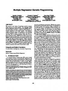
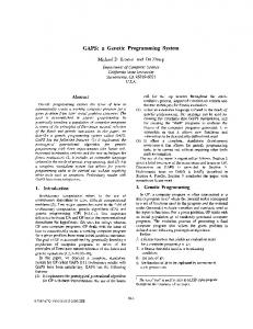
Fig. 1. Trees represented in s-expression (AND OR A B NOT C) and (AND NOT A OR B C).

of the complete program tree is also used to update the fitness of its tree nodes and subtrees. A tree node evolves on its own by reproducing instructions of good fitness and removing instructions of bad fitness. This paper is organized as follows. Section II reviews some of the related GP algorithms. Section III describes the representation and algorithm of IMGP in detail. Section IV presents the experiments on the benchmark GP problems. Section V gives an application example of IMGP for classification problems and the experimental results. Section VI provides the conclusion.

1037

an execution path. There can be multiple execution paths in a grid. Executing the program is evaluating the functions and terminals, following the execution paths in parallel. Crossover and mutation are performed on the level of subgraphs. Cartesian GP [25] is based on a grid of function nodes. The program is represented as a sequence of groups of indices. Each group of indices corresponds to a function node in the grid, and it consists of three indices for the inputs, and one index for the function node. Crossover and mutation are used to modify the index sequence. Genetic parallel programming [21] evolves a parallel program on a multi-arithmetic-logic-unit processor. A parallel program is a sequence of parallel instructions. A parallel instruction consists of several subinstructions, which are simultaneously executed. Genetic parallel programming is observed to evolve parallel programs with less computational effort than the equivalent sequential programs. Grammatically based GP (GGP) [40], [41] indirectly represents programs. It uses a set of grammar rules to generate a population of grammar derivation trees. The sequence of the leaves of the tree is interpreted as a program. It also employs some advanced mechanisms, such as type control, grammar modification, merit selection, and encapsulation.

II. R ELATED W ORK A. Genetic Programming

B. Genetic Programming With Statistics

In this paper, we shall focus on general GP algorithms, which are capable of solving the benchmark problems commonly tested in GP research. CGP [19] is the original standard GP. It represents a program as a tree that is encoded in a LISP-like s-expression. Fig. 1 shows two examples. A tree is composed of tree nodes of functions and terminals. Executing a program is recursively traversing the tree in postorder. CGP crossover is selecting two crossover points in two parental trees, respectively, and exchanging the corresponding subtrees. Similarly, CGP mutation is selecting a mutation point in the parent and replacing the subtree with a new randomly generated subtree. Strongly typed GP [26] enforces data type constraints in CGP to manipulate multiple data types. It is thus able to avoid searching in the solution space involving inappropriate data types. It also employs generic functions and generic data types to make it more powerful and practical. Linear GP [1] represents the program as a sequence of machine codes executed on a virtual register machine. The program receives the inputs from the registers and puts the output in a specified register. The crossover is swapping the segments of the codes between two crossover points in the parents. Mutation is replacing an instruction code with a new randomly generated one. Evaluating the program is executing the codes sequentially on the register machine. Stack-based GP [27] is similar to linear GP, as it represents the program in a sequence of functions and terminals. However, it is executed on a stack-based virtual machine, and its instruction set includes the stack operations, e.g., POP & PUSH. It uses simple two-point crossover and one-point mutation. Graph GP [28] encodes the program in a grid of functions and terminals. Some of the nodes in the grid are connected with directed links. A link indicates the order of execution, and a sequence of continual links forms

IMGP uses an IM to maintain the fitness of functions and terminals of the tree nodes, and it extracts new program trees out of the IM. There is some related work that also keeps the statistical data of the individuals and generates individuals from data structures other than populations. Probabilistic incremental program evolution (PIPE) [33] maintains a probability tree. A tree node is a vector of the probabilities of the functions and terminals on the tree node. In each generation, PIPE creates a population by constructing trees according to the probability tree and updates the probability tree with the information of the best individual in the population. However, updating the probability tree only with the best individual may not be able to express the information of the rest of the population. In addition, it ignores the interdependencies between the tree nodes. Competent GP [34] combines compact genetic algorithm [17] and PIPE as a multivariate probabilistic model of program trees. The major contribution is that it partitions the tree into subtrees and builds a probabilistic model for each subtree. Therefore, it is able to calculate not only the probabilities of the tree nodes, but also the probabilities of the subtrees. However, it incurs high computation overhead as it calculates the complexity of each possible subtree to identify good building blocks. Estimation of distribution programming (EDP) [42] estimates the probability distribution model in the form of a Bayesian network to capture the relationship between the tree nodes in GP. It is observed that while CGP produces deep trees, EDP is good at wide trees. To search for more different tree topologies, it is suggested that multi-Bayesian networks be used, though it incurs higher computation cost. Grammar-model-based program evolution (GMPE) [36] evolves programs with a probabilistic contextfree grammar. It associates each grammar rule with a production probability. It uses the grammars to generate a population

1038

IEEE TRANSACTIONS ON SYSTEMS, MAN, AND CYBERNETICS—PART B: CYBERNETICS, VOL. 38, NO. 4, AUGUST 2008

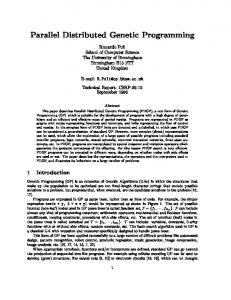
of new individuals and updates the grammars with the good individuals in the population. A grammar generates a single node or a subtree, so it is able to maintain the information of subtrees as well. However, the grammar has no information of the position in the whole tree, so the position of its derivative (node or subtree) in the tree is not fixed. In addition, a grammar could generate two totally different subtrees, depending on the successive grammars applied. Estimation of distribution algorithms for GP [6] is similar to GMPE. It employs a probability distribution over grammars to generate new programs. Complex production rules or subfunctions can be introduced by using transformation to expand one production rule into another production rule so as to express a high order of dependencies. However, learning advanced production rules with the proposed greedy algorithm can take a lot of time. Program evolution with explicit learning (PEEL) [35] uses search space description table (SSDT) to describe the solution space. Ant colony optimization [5] is the learning method to update the stochastic components of SSDT. Grammar refinement by splitting certain rules in SSDT is employed to make individuals focus on the promising solution area. Grid ant colony programming [32] uses ant colony metaheuristic [11] to guide a population of ants on a grid of functions or terminals. The tour of an ant is interpreted as a program. III. IMGP CGP is a high-dimensional combinatorial optimization problem if tree nodes are treated as variables. To apply the divideand-conquer methodology, we propose a new framework called IMGP. IMGP evolves tree nodes separately while taking into account their interdependencies in the form of subtrees. IMGP maintains an IM to keep the fitness of functions and terminals in tree nodes, and it uses a new kind of fixed-length expression to represent a program tree. IMGP extracts a program tree from an IM by selecting a function or terminal of high good fitness for each possible tree node. After the program tree is evaluated, IMGP updates the fitness of corresponding functions or terminals in the IM. A. Representation Rather than using an s-expression as CGP [19], IMGP uses an hs-expression. An hs-expression is mapped to a program tree. An hs-expression is a 2D+1 − 1 long array to store a binary tree of depth D at most. Every possible node in the tree has a corresponding element in the array, even if the node does not exist. The relation between the elements in an hs-expression is similar to that used in the array of heap sort, but the “largerthan” relation is changed to the “parent-of” relation. The tree root is element 0 in the hs-expression. For the kth element in the hs-expression, its left and right children are the 2k + 1th and 2k + 2th elements, respectively. If it has no child, the corresponding elements are set to −1 instead. Therefore, the elements in the first half of the array can either be functions, terminals, or empty, while the elements in the second half of the array must either be terminals or empty. Fig. 2 shows two examples. Unlike the trees represented by an s-expression, the

Fig. 2. NOT OR

Trees represented in hs-expression (AND OR NOT A B C -1) and (AND A -1 B C).

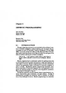
trees represented by an hs-expression of the same length have exactly the same shape if −1 is viewed as a virtual node. Another difference is that the elements at the same locus in hsexpressions always correspond to the nodes at the same position in program trees. In comparison to this, genetic expression programming [14] also uses a fixed-length string to represent a tree, and some of its elements may not appear in the tree. However, when the arity of a tree node changes, the positions of its subtree and its sibling change drastically. An hs-expression can easily be extended to represent trees of more than two branches. To represent an m-branch tree, an hs-expression is an mD+1 − 1 long array. For the kth element in the hs-expression, its children are the m · k + 1th, m · k + 2th, . . . , m · k + mth elements. In IMGP, there is no explicit population. Instead, it maintains an IM to store all the possible instructions used in a program tree. While CGP generates new program trees from existing program trees, IMGP extracts new hs-expressions from the IM, which are mapped to program trees. The cells in the IM are data structures consisting of instructions and related information. A row in an IM corresponds to an element in the hs-expression, and, hence, a tree node in a program tree. The cells in a row stores all the possible instructions that can be used in the corresponding tree node. The mapping between the IM and program trees is the same as the mapping between an hsexpression and a program tree: row 0 corresponds to the root of the program tree. Recursively, for the kth row corresponding to a tree node, the 2k + 1th and the 2k + 2th rows correspond to the left and right children of the tree node, respectively. The height of the IM is the same as the length of the hs-expression, i.e., H = 2D+1 − 1. A row contains multiple instances of any type of instructions, and therefore, the width W of the IM is the number of instructions in a row. The lower part of the IM, i.e., the part from row H/2 to row H, contains only terminals since they correspond to the tree leaves. Fig. 3 shows an example of an IM and an hs-expression extracted from it. Basically, the element at locus k in the hs-expression is extracted from row k in the IM. The details are described in Section III-B. In addition to an instruction of function or terminal, a cell in the IM also keeps some auxiliary data. The pseudocode of its internal data structure and the initial values are shown in Fig. 4. The data structure also stores the information of its best subtree. instruction is the operation code of the instruction. eval_num is the number of times that the instruction has been evaluated. best_f itness and avg_f itness are the best and the average fitness of the instruction. best_f itness is also the fitness of the best subtree of the instruction. lef t_branch and right_branch are the left and right branches of the best subtree. These fields

LI et al.: INSTRUCTION-MATRIX-BASED GENETIC PROGRAMMING

1039

Fig. 3. IM and an hs-expression extracted from it. IM keeps multiple instructions for each element of the hs-expression. An element of the hs-expression is extracted from the corresponding row in the IM. The cells in bold typeface are the extracted elements.

Fig. 4. Pseudocode of the internal data structure of the cell in the IM, which shows the initial values of the fields. The field instruction can be either a function or a terminal. M AX_F IT N ESS and 0 are the maximal and minimal possible fitness, respectively. −1 means that there are no links for the left and right children of the tree node at the beginning.

keep some information of the fitness landscape of the tree node, and they are used in the evolution of the tree node. Their specific usage is explained in detail in Section III-B. Please note that in IMGP, the smaller the fitness is, the better it becomes. B. Algorithm Algorithm 1 is the main program of IMGP, where G is the maximal number of generations, and P is the number of individuals in each generation. It divides a complete tree into separate tree nodes, calculates the fitness of the tree nodes to evolve them separately, and combines the optima of the tree nodes into a complete program tree. In each generation, IMGP repeatedly runs the following steps. First, IMGP extracts two individuals from the IM and calculates their fitness. Then, IMGP performs crossover and mutation on them and calculates the fitness of their offspring. After evaluating an individual, IMGP updates the corresponding cells in the IM with the fitness of individual. At this point, IMGP deletes all of the individuals because their information has already been stored in the IM. A generation finishes after IMGP evaluates P individuals. Then, IMGP uses matrix shuffle to replace cells of bad fitness with those of good fitness in the IM. The best individual is reported as the optimal program after G generations. Algorithm 1: The Main Program of IMGP Output: the best individual initialize IM for gen from 0 to G do num ← 0; while num < P do extract two individuals i and j from IM; calculate their fitness respectively; update their cells in IM with the fitness; if crossover i with j successfully then evaluate the offspring and update its cells; else if mutate i successfully then evaluate the offspring and update its cells;

Fig. 5. Steps of extracting (AND OR NOT A B C -1) from the IM in Fig. 3. For each tree node, IMGP selects two instructions in the corresponding row of IM randomly, compares their average and best fitness, and extracts one of them probabilistically. After extracting a tree node, IMGP recursively extracts its left and right children.

end if crossover j with i successfully then evaluate the offspring and update its cells; else if mutate j successfully then evaluate the offspring and update its cells; end num ← num + the number of individuals evaluated; end shuffle IM; end

1) Individual Extraction: IMGP extracts the tree nodes from the IM and combines them into a complete tree. Algorithm 2 is the function to extract an individual. First, IMGP constructs an empty hs-expression filled with −1 and aligns it vertically with the IM. It starts to extract the instruction of the tree root from row 0 and puts it at locus 0 in the hs-expression. Then, IMGP continues to extract the rest of the program tree recursively. The instruction of a tree node is extracted from the corresponding row using binary tournament selection, and then, the extracted instruction is placed at the corresponding locus in the hs-expression. Binary tournament selection is comparing the fitness of two randomly selected instructions and selecting one of them probabilistically. If the extracted instruction at locus k is a function, IMGP proceeds to extract its left child from the 2k + 1th row and its right child from the 2k + 2th row. It does so recursively until all the branches are completed. In Fig. 3, the words in bold italic typeface are the extracted instructions, and the completed hs-expression is on the right. The corresponding tree is depicted on the left in Fig. 2. The details of extracting (AND OR NOT A B C −1) from the IM is shown in Fig. 5. Algorithm 2: Extract Individual Input: individual, IM, locus, subtree Output: individual best ← false;

1040

IEEE TRANSACTIONS ON SYSTEMS, MAN, AND CYBERNETICS—PART B: CYBERNETICS, VOL. 38, NO. 4, AUGUST 2008

if subtree = −1 then individual[locus] ← subtree; CELL ← IM [locus, individual[locus]]; best ← true; else individual[locus] ← T ournament(IM, locus); CELL ← IM [locus, individual[locus]]; _f itness then if Random(1) < 1 − CELL.best CELL.avg _f itness best ← true; end end if best = true and CELL.instruction is function and CELL.lef t_branch = −1 and CELL.right_branch = −1 then Extract(individual, IM, locus∗ 2 + 1, CELL.lef t_branch); Extract(individual, IM, locus∗ 2 + 2, CELL.right_branch); else Extract(individual, IM, locus∗ 2 + 1, −1); Extract(individual, IM, locus∗ 2 + 2, −1); end

The best subtree of an instruction is its subtree in the best individual that it has ever been extracted in. After a tree node is extracted, IMGP occasionally checks whether the best subtree of the selected instruction should be extracted as a whole so that the tree nodes in the best subtree are extracted directly without further binary tournament selections. How often it does so depends on the best and the average fitness of the instruction. Equation (1) is the probability of extracting the best subtree. The bigger the difference between them is, the more likely its subtree will be selected. The reason is that if the best fitness is much better than the average fitness, the tree constructed with the best subtree is likely to be much better than the tree constructed without it. Since tree nodes are highly interdependent with respect to the fitness in GP, best subtrees keep part of the interdependence information between the tree nodes in the IM, i.e., probbest = 1 −

best_f itness . avg_f itness

(1)

In the binary tournament selection, IMGP randomly selects two candidate instructions, compares their fitness, and selects the better one probabilistically. An instruction is extracted either separately or together with its best subtree. Therefore, when we compare the fitness of two candidate instructions, we should not only compare their average fitness, but consider their best fitness as well. Equation (2) calculates the expected fitness of an instruction. It considers the probability of selecting its best subtree, and in that case, we should use the best fitness. The traditional binary tournament selection always selects the better one, so the worst instruction in the IM is never selected. To be less greedy, we use roulette wheel selection [15] to select one of the two instructions based on their expected fitness, which is defined by E(f itness) = probbest ∗ best_f itness + (1 − probbest ) ∗ avg_f itness. (2)

Extracting individuals makes IMGP avoid being trapped in a small solution area. In CGP, when an individual is changed by crossover or mutation, it replaces only a subtree with a new one, so the offspring is still in the neighborhood of the parent. Therefore, the solution space that CGP searches is largely determined by the initial population. However, IMGP does not generate an individual from an existing parent. It extracts a completely new individual from the IM, and thus, the new individual bears slim similarity with the previous individuals. Therefore, IMGP searches a relatively large solution space, and the extracted individuals together have high diversity. In addition, there are multiple copies of any type of instructions in a row in an IM, and each copy has different fitness and subtrees. Even if an instruction has a bad fitness copy, it might still be selected due to another copy of good fitness. Therefore, IMGP is relatively robust to local optima. 2) Instruction Evaluation: In IMGP, an individual is evaluated using the postorder recursive routine. To evaluate a function node, it takes the evaluation of its left and right children as the inputs. To evaluate a terminal node, it evaluates the corresponding program input. Since the individual is discarded right after evaluation and reproduction, it cannot carry along its fitness as in CGP. Instead, the fitness is fed back to its corresponding cells in the IM so that it can be used in extraction later. The feedback comes in two ways. 1) In (3), the new fitness, i.e., f itness , is averaged with the old fitness, i.e., f itness. The evaluation number eval_num is incremented by one. With this method, we know how good the instruction is on the average. We have f itness =

f itness ∗ eval_num + f itness . eval_num + 1

(3)

2) If the new fitness is better than the best fitness of the instruction, its best fitness is updated, and its left and right branches are changed to those in the current individual accordingly. This actually keeps good subtrees in the IM together with their fitness. The second point is very important. As shown in [37], a new building block is unlikely to survive in the next two generations, even if the individual constructed with it has average fitness. In IMGP, whenever a good subtree is identified, it is remembered immediately. We believe that all the individuals contain useful information about the problem. Therefore, IMGP updates the IM not only with the good individuals, but with all the extracted individuals as well, regardless of their fitness. For most of the related algorithms discussed in Section II-B, they update their models only with good individuals and ignore bad individuals. This would make some of the bad tree nodes spuriously good in the models because they happen to be in the good individuals. On the contrary, updating the IM with bad individuals decreases the fitness of the bad tree nodes. Tree nodes and subtrees can also be regarded as schemata, and thus, IMGP actually evolves schemata directly [22]. 3) Genetic Operators: In IMGP, crossover and mutation are similar to those in CGP. However, as IMGP keeps the fitness of the tree nodes in the IM, it is able to perform crossover and

LI et al.: INSTRUCTION-MATRIX-BASED GENETIC PROGRAMMING

Fig. 6.

1041

Crossover in IMGP. The left subtree in the first individual is replaced with its better counterpart in the second individual.

mutation in a heuristic way. According to the building block hypothesis [15], small good building blocks are spread among the individuals and recombined into large good building blocks. Therefore, we believe that combining subtrees of high good fitness is likely to produce individuals of good fitness. When IMGP performs crossover on individuals, it replaces a subtree in one parent only, with a better counterpart in the other parent, so that the offspring is likely to be better. In mutation, IMGP selects a mutation point in the current individual and replaces the original subtree with a new subtree extracted from the IM. The crossover is similar to context-preserving crossover [10] because the two subtrees of the parents must be in the same position to reduce the macromutation effect of the standard crossover [1]. However, unlike the crossover used in other GP algorithms, the crossover in IMGP is asymmetric. When IMGP tries crossover between individual i and individual j, it picks one of the two branches on the roots in both individuals at random and replaces the subtree of i with that of j if the latter has better fitness than the former. Otherwise, IMGP recursively tries crossover on the roots of the picked branches. Fig. 6 shows an example. Please note that crossover would fail when it could not find a better subtree to replace the original one. 4) Matrix Shuffle: CGP converges by spreading good instructions over the population to reproduce good individuals. IMGP starts with extracting program trees from the IM at random, so it samples different solutions in the huge solution space. In the evolution, it is important for IMGP to sample program trees that are similar to the previously extracted good program trees. However, there is no explicit population in IMGP since it extracts an individual and discards it later. To ensure that the individuals extracted in the later generations have good instructions, the IM should be populated with good instructions. IMGP uses matrix shuffle to propagate good instructions in the IM and, consequently, to increase the probability of extracting them together in the same program tree. It shuffles the IM row by row. Algorithm 3 shows how it shuffles a row. It selects a certain number of pairs of cells in a row, and for each pair, it replaces the worse one with the better one in terms of both the best and the average fitness. Consequently, while the IM evolves, good instructions emerge to dominate the rows in the IM, and the copies of bad instructions decrease. Algorithm 3: Matrix Shuffle Input: IM, the current row to be shuffled Data: F ∩ T is the function and terminal set for instruction ∈ F ∩ T do

Count[instruction] ← the number of instruction in IM[row]; end while si < SU CCESS and ti < T RIAL do ti ← ti + 1; i, j ← Random(W ); Ci ← IM [row, i]; Cj ← IM [row, j]; if Ci.avg_f itness < Cj.avg_f itness and Ci.best_f itness < Cj.best_f itness and Count[Ci.instruction] < CON V ERGEN CY and Count[Cj.instruction] > DIV ERSIT Y then IM [row, j] ← IM [row, i]; si ← si + 1; end if Cj.avg_f itness < Ci.avg_f itness and Cj.best_f itness < Ci.best_f itness and Count[Cj.instruction] < CON V ERGEN CY and Count[Ci.instruction] > DIV ERSIT Y then IM [row, i] ← IM [row, j]; si ← si + 1; end end

In CGP, as the population converges, the majority of the individuals have more or less the same instructions, while the other instructions die out. It is also hard to maintain the diversity of the population because measuring the distance between individuals is difficult. However, IMGP evolves on the level of instructions, so it is possible to maintain the diversity of the instructions. In matrix shuffle, when a good instruction IM [row, i] replaces a bad instruction IM [row, j], where i and j are the indices for the two instructions, IMGP needs to check two constraints: Count[IM [row, i]] < CON V ERGEN CY and Count[IM [row, j]] > DIV ERSIT Y . To discourage convergence, CON V ERGEN CY should not be too high, and to enhance diversity, DIV ERSIT Y should not be too low. In the current implementation, we use CON V ERGEN CY = W/2 and DIV ERSIT Y = 2. As shown in [7], the edit distance, i.e., the difference between a program tree and the best program tree, generally decreases after the early generations in CGP. It is thus good to keep the edit distance not too small to enhance the diversity of the population. Basically, matrix shuffle prohibits good instructions from reproducing themselves too many times and reserves a minimum number of bad instructions. This thus maintains the diversity of the instructions in the IM easily and effectively.

1042

IEEE TRANSACTIONS ON SYSTEMS, MAN, AND CYBERNETICS—PART B: CYBERNETICS, VOL. 38, NO. 4, AUGUST 2008

TABLE I EXPERIMENT SETTINGS OF IMGP AND LILGP ON THE BENCHMARK PROBLEMS

C. Algorithm Complexity In addition to the normal genetic operators and fitness evaluation in CGP, IMGP introduces additional overhead of extracting individuals, updating the IM, and shuffling the IM. First, the time complexity of genetic operators is O(H), where H is the height of the IM, i.e., the size of the program tree. Second, extracting individuals and updating the IM need to go through all the instructions in the program trees, so the complexity is also O(H). Third, the complexity of shuffling the IM is of the size of the IM, i.e., O(W H), where W is the width of the IM. Fourth, the time complexity of evaluating the fitness is O(N H), where N is the number of times to traverse tree programs. For some problems, N is the number of training cases. Suppose IMGP runs for G generations and extracts P program trees in each generation, then the overall time complexity is O(GP H + GW H + GP N H). The time complexity of CGP is O(GP H + GP N H). In fact, for both IMGP and CGP, most of the computation cost is spent in evaluating the fitness, whose complexity is O(GP N H). For program tress with similar sizes, the time complexity of IMGP is only slightly larger than that of CGP. However, the space complexity of IMGP is smaller than that of CGP. The major part of the space complexity of CGP comes from the population of individuals, i.e., O(P H), while the major part of the space complexity of IMGP comes from the IM, i.e., O(W H). Usually, W is on the order of hundreds, while P is on the order of thousands. IV. E XPERIMENT This section describes the experiments and the results of IMGP. First, we ran IMGP and CGP on the benchmark GP problems and compared the results. Second, we applied IMGP on the problems tested in the related algorithms in Section II-B and compared the results. A. Comparison With Canonical Genetic Programming This section compares the performance of IMGP and CGP on four benchmark problems [19]. The first problem is the symbol regression problem that searches for a mathematical expression y = x4 + x3 + x2 + x, where x is an integer uniformly and randomly generated from the range [0, 20). The fitness used is the hit count, which is incremented by one if the difference between the program output and the correct result is larger than a predefined threshold. The second problem is to discover the even-5-parity expression ¬(a ⊕ b ⊕ c ⊕ d ⊕ e). The training cases are all the 25 combinations of the five binary variables. The fitness is calculated

as the sum of the wrong results produced by the individual program. The third problem is the artificial ant on Santa Fe Trail. Executing the optimal program repeatedly enables the ant to eat all the 89 food pellets on the trail within 400 steps. The number of the food not eaten by the ant is used as the fitness. The fourth problem is Boolean 11-multiplexer. Among the 11 variables, three are used as the address to select the output from one of the other eight variables. However, GP has no idea of which variables are the address. The training cases are all the 211 combinations of the 11 binary variables, and the fitness is the number of incorrect output. Table I lists the parameter settings used in the experiments. IMGP has no population, but for convenient comparison with CGP, we refer to the number of the individuals evaluated between matrix shuffles (generations) as the population size, i.e., P in Algorithm 1. Please note that in Artificial Ant and 11-Multiplexer, some functions require three arguments, which means that the maximum branches of a node is three instead of two. Therefore, the IM height and the hs-expression length is increased to (3D+1 − 1)/2, where D is the maximal level of a program tree. To determine an acceptable size of the IM, we executed IMGP of different sizes on a small number of the training cases for a few generations. By observing the fitness of the best program trees, we could determine which size was likely to produce a good solution. We used lilgp [44] as CGP. For fair comparison, the ephemeral random constant (ERC) was removed from lilgp. The tournament size was two. The population size and the number of generations were set as in Table I. The other parameters were the same as in [19]. Both lilgp and IMGP used the same random seeds, which themselves were randomly generated. For each problem, we ran IMGP and lilgp 20 times with 20 different random seeds. Fig. 7 shows the plots of the average fitness of the best individuals from generation 1 to generation 100 for the four problems. Table II shows the numerical experimental results of IMGP, including the success rate, the fitness of the best program tree, the number of fitness evaluations, and the size of the best program tree. In symbol regression, IMGP found the solution in all the 20 runs compared with 17 successful runs in lilgp. In terms of the average fitness of the best individuals, IMGP also converged faster than lilgp. In even-5-parity, IMGP found the solution in three runs, however, lilgp failed to find the solution in any of the 20 runs. Regarding the convergence speed, IMGP also outperformed lilgp significantly, as its average best fitness was 2.4, while lilgp’s was nearly twice of that. In 20 artificial ants, IMGP found 12 ants eating up all the food pellets. lilgp could not find any successful ant, and the average fitness of its best individuals was 31.8, which is far from 0. In an 11-multiplexer,

LI et al.: INSTRUCTION-MATRIX-BASED GENETIC PROGRAMMING

Fig. 7.

1043

Average fitness of the best individuals of IMGP and lilgp through generations on the four testing problems. TABLE II NUMERICAL EXPERIMENTAL RESULT OF IMGP ON THE BENCHMARK PROBLEMS. IT SHOWS THE SUCCESS RATE, THE FITNESS OF THE B EST I NDIVIDUALS , THE N UMBER OF P ROGRAM E VALUATIONS , AND THE N UMBER OF T REE N ODES

TABLE III COMPARISON OF THE RUNNING TIMES OF IMGP AND CGP ON THE FOUR BENCHMARK PROBLEMS. THE TIME UNIT IS SECONDS

IMGP found the perfect multiplexer for 13 times out of 20 runs, while lilgp failed all the time. The average best fitness of IMGP was also much better than that of lilgp, although their fitness in the first generation were almost the same. We have also compared the running times of IMGP and CGP in Table III. They were executed on a Linux workstation of Pentium 2.2 GHz. Except for the even-5-parity problem, the running time of IMGP is shorter than that of CGP. This is expected, since IMGP has much larger success rates than CGP. IMGP stops early before the final generation 100 when it finds a perfect solution. For the difficult even-5-parity problem, the IM has many rows so that the tree programs have many levels. Therefore, IMGP is slower than lilgp on even-5-parity. B. Comparison With Related Algorithms We had also run IMGP on the problems tested by the related algorithm and compared the results. However, it is difficult to compare the results precisely, as some of the papers gave the results only in the figures without the exact numerical values. Therefore, we will have to resort to the problems whose results were reported in numbers in other papers. The experiment settings were the same as in the related algorithms described in Section II-B. The 6-bit parity problem is similar to even-5-parity. It has six Boolean arguments, and it returns true if the number of true arguments (1s) is odd and false otherwise. However, other than using the Boolean function set, it uses a real-valued function set

{+, −, ×, %, sin, cos, exp, r log}, where r log is the protected log that returns the log of the absolute value of the argument. The output of the program is mapped to true if it is larger than 0 and false otherwise. We executed IMGP for this problem in 20 independent runs. The result is compared to that of PIPE [33] and CGP in Table IV. As can been seen, IMGP achieves 100% success rate, and it requires a much smaller number of program evaluations. The max problem has a single input with a value of 0.5 and two functions + and ×. The purpose is to find a tree with maximum fitness under the tree size constraint. Obviously, the optimal tree is a full tree, whose nodes on the two levels right above the terminals are + to produce the value of 2, and the other nodes on the top are × to multiply all of the 2’s. In this experiment, the maximum tree depth is 7, so the maximum fitness is 65 536. The result compared to GMPE [36] and CGP is reported in Table V. With approximately the same number of evaluations, when GMPE converges, it has a higher success rate than IMGP. However, if IMGP keeps running until 100 generations, its success rate increases to 95%. Both IMGP and GMPE outperform CGP. Function regression is used to search for the function shown in (4). The fitness cases were sampled at 101 equidistant points in the interval [0, 10]. The fitness is not the hit count but the sum of the differences between the outputs and the correct answers. The fitness of the best individuals of IMGP are compared to those of PEEL [35] and GGP [40] in Table VI. IMGP gets a smaller error and a smaller standard deviation. Although the minimum errors of PEEL and GGP are smaller than that of IMGP, their median and maximum errors are much larger than those of IMGP. Therefore, if we run IMGP, PEEL, and GGP ten times, the results of IMGP will be less variant than those of PEEL and GGP. If we run the programs only once, the result of IMGP is expected to be better than that of GGP and PEEL. We have f (x) = x3 × e−x × cos x× sin x× (sin2 x× cos x − 1).

(4)

1044

IEEE TRANSACTIONS ON SYSTEMS, MAN, AND CYBERNETICS—PART B: CYBERNETICS, VOL. 38, NO. 4, AUGUST 2008

TABLE IV EXPERIMENTAL RESULTS OF IMGP, PIPE, AND CGP ON THE SIX-BIT PARITY PROBLEM. IT SHOWS THE SUCCESS RATE, THE N UMBER OF P ROGRAM E VALUATIONS , AND THE N UMBER OF T REE N ODES

TABLE V EXPERIMENTAL RESULTS OF IMGP, GMPE, AND CGP ON THE MAX PROBLEM. IT SHOWS THE SUCCESS RATE AND THE N UMBER OF P ROGRAM E VALUATIONS

TABLE VI EXPERIMENTAL RESULTS OF IMGP, PEEL, AND GGP ON FUNCTION REGRESSION. IT SHOWS THE FITNESS OF THE BEST INDIVIDUAL

V. A PPLICATION FOR C LASSIFICATION The problem of classification has been a major task of machine learning and data mining. Basically, given a set of training data, we learn a classifier so that it can be used to classify new data. Typical classifiers include decision trees (DTs) [31], neural networks [3], and support vector machines (SVMs) [8], etc. GP can also be used to evolve classifiers in the form of programs. GP has a few favorable features for classification, such as the variable-length representation and the population of different solutions [12], [23], [38]. First, the structures of many traditional classification models are fixed: the major task of learning is to find the proper parameters of the models. Because a variable representation of classifiers is adopted in GP, it bears more freedom to find appropriate model structures than fixed representations. Second, the results of some traditional learning algorithms depend on the initial parameters of the models. In GP, the population contains many individuals, so GP has a better chance of finding the appropriate structures and the parameters of the models. In this section, we will first describe a direct implementation of IMGP for binary class classification problems. Then, we will present an extension of IMGP for multiclass classification problems. The experimental results are also reported. A. IMGP for Classification In a binary classification problem, we are given a training data set X that consists of N samples {xi |i = 1, . . . , N }. A sample xi has M attributes {xij |j = 1, . . . , M }. For each sample xi , there is a target class ti . Given a sample xi , a classifier predicts its class as y i . The task of the classifier learning algorithm is to find a classifier of minimal error. In

this paper, the sum of squared error function is only applied on the misclassified data as follows: N


1
(ti − yi )2 E= 2 i=1

(5)

where N  is the number of misclassified data. Suppose the instruction set in CGP is {x1 , . . . , xm , +, −, ×, /}, the program tree is actually a mathematical formula. The class boundary can be represented by a mathematical formula. For a binary class problem, the program tree receives the attributes of a sample as the inputs. If the output of the program tree is positive, the sample is assigned class 1; otherwise, it is assigned class 2. The classification error on the training data is used as the fitness. As a variant of CGP, IMGP can also be used for classification problems. As described in Sections III and IV, we envisage that IMGP will be more efficient and more effective than CGP. We introduce constant instruction (CI) in the instruction set of IMGP. A CI is used as a terminal of constants, which is similar to the adjustable parameters in other kinds of classifiers. CGP uses the ERC as a constant. ERC is instantiated to a random number in the initialization of CGP, and the number is fixed in later generations. In IMGP, because a CI will be extracted into different individuals, it should change the constant during evolution. A CI has two constants, i.e., the random constant (RC) and the best constant (BC), corresponding to its average and best fitness, respectively. BC is used when the CI is used in the best program tree for testing on unknown data. RC is assigned a new random number whenever it is extracted in a new individual. The new value of RC replaces the value of BC if the new individual has better fitness than the best fitness of the CI. In contrast to CI in IMGP, ERC does not change during evolution, even if the change will lead to a better constant, given the structure of the program tree. As mentioned in [9], various approaches have been proposed to change a constant in the evolution. However, they are only mutation on the constant disregarding the current individual. In neural networks [3] and SVMs [8], the structure of the model is given beforehand, and the learning process is adjusting the model parameters to minimize the error function. GP can be viewed as searching for the structure of the model and the parameters of the model simultaneously. It is thus possible to change the parameters without changing the structure to achieve better fitness. If the error in (5) is used as the fitness and the structure of the program tree is fixed, the fitness is actually a continuous function of constants. Therefore, IMGP can modify the constants of a program tree to obtain a lower classification error. As in neural networks, IMGP uses gradient descent [3] to find the optimal

LI et al.: INSTRUCTION-MATRIX-BASED GENETIC PROGRAMMING

1045

TABLE VII COMPARISON OF IMGP AND G3 P ON THE FOUR UCI BENCHMARK CLASSIFICATION PROBLEMS. DT, FRBS, ANN, AND PETRI ARE THE FOUR GP APPROACHES. WE COMPARE THE TRAINING AND TESTING ERRORS IN THEIR BEST AND AVERAGE RESULTS. THE ERRORS ARE REPORTED IN PERCENTAGES

constants. In the method of gradient descent, a constant is changed according to the following partial derivative of MSE:


N
η ∂E ∂yi c =c− =c+η (ti − yi ) 2 ∂c ∂c i=1 

(6)

where η is the learning rate, c is the vector of the constants, and yi is the output of the program tree, given the sample xi . Given a mathematical formula represented by a program tree, we can calculate its partial derivative with respect to the constant. Suppose the formula is a composite function y = (f ◦ (g, h))(c), where the function f takes two arguments of the functions g and h. The derivative of f with respect to c is ∂y/∂c = (∂f /∂g)(∂g/∂c) + (∂f /∂h)(∂h/∂c). A simple example is (a/b) = (∂/∂a)(a/b)a + (∂/∂b)(a/b)b = (1/b)a − (a/b2 )b . Therefore, we can calculate ∂y/∂c by traversing the program tree in postorder. However, we need to calculate both the outputs and the partial derivatives of the tree nodes, so the computation cost is multiplied by the number of constants. To save computation, gradient descent is not used on every program tree. It is used only when IMGP finds a new best program tree. Gradient descent for GP was also used in [43]. It used gradient descent for all the individuals that would be quite time consuming. One of the major concerns of classification problems is generalization [18]. Due to the noise in the training and the testing data, a classifier that works well on the training data may not be so accurate on the testing data. A reason for the performance degradation is that the classifier is so complex that it classifies noisy data unnecessarily. A common approach to enhance generalization is to trade the classification accuracy for the model complexity. In IMGP, we add a penalty of the tree size with the original classification error as the fitness shown in the following: f itness = error + w

tree size M _ROW

(7)

where w is a small positive constant that controls the weighting of the tree size. Because the classification error is always less than 1, the tree size is normalized with the maximum tree size, i.e., M _ROW . In calculating the tree size, IMGP does not count the terminal nodes, since only the functions contribute to the complexity of the program. The linear functions of + and − represent linear models that are simple enough, so

they are not counted either. Therefore, in the instruction set {x1 , . . . , xm , c, +, −, ×, /}, only the nonlinear functions × and / are counted in the tree size. We ran IMGP on four benchmark binary classification problems in the University of California, Irvine (UCI) repository [4], i.e., breast cancer Wisconsin (Cancer), heart disease (Heart), Pima Indians diabetes (Pima), and horse colic (Horse). We adopted a fivefold method, and for each fold, IMGP was run for 20 times of different random seeds, so there were altogether 100 independent runs. We quote the results of grammar-guided GP (G3 P) [38] for comparison. G3 P was used to evolve four kinds of classifiers: 1) decision tree (G3 P-DT); 2) fuzzy-rule-based system (G3 P-FRBS); 3) artificial neural network (G3 P-ANN); and 4) fuzzy Petri net (G3 P-FPN). Both G3 P and IMGP used populations of 2000 individuals, and the maximum generations are 100. Table VII shows the results of the training and testing errors, which are reported in their best and average. For the average training errors, the results of IMGP are comparable to the four other algorithms. This verifies the effectiveness of IMGP on the training data. The testing error is a more important measure of performance than the training error. IMGP generalizes very well compared to the four other algorithms. IMGP is robust to different random seeds, because it gets the lowest average testing errors on the four problems. For the best testing error, IMGP gets the second lowest best testing error on the Cancer problem, and its best testing errors are the lowest on the three other problems. We have also compared IMGP to some traditional classifiers other than GP, including DTs, neural networks, and SVMs. The DT that we used was C5.0 [30], which is the state of the art of DTs for classification. The SVM that we used was LIBSVM [13]. We activated its cross validation on the training data to determine the parameters of the kernel function. An SVM is a deterministic algorithm, so we need to run it only once. We have implemented the neural network based on the functions provided by Matlab. We used cross validation on the training data to choose the number of hidden neurons, and then an automated weight decay learning was used to train the neural network on the whole training data. A neural network is sensitive to the initial weights, so we ran the program ten times with different random seeds. A DT is a deterministic algorithm, but C5.0 uses random fivefold for training and testing, so we executed C5.0 ten times as well. The testing errors are reported in Table VIII. For the convenience of comparison, the result of the SVM is treated as both the best and the average results.

1046

IEEE TRANSACTIONS ON SYSTEMS, MAN, AND CYBERNETICS—PART B: CYBERNETICS, VOL. 38, NO. 4, AUGUST 2008

TABLE VIII COMPARISON OF IMGP, DT, NEURAL NETWORKS, AND SVM ON THE FOUR UCI BENCHMARK PROBLEMS. THE BEST AND AVERAGE TESTING ERRORS IN PERCENTAGES ARE REPORTED. FOR THE DETERMINISTIC ALGORITHMS, i.e., DT AND SVM, THE B EST AND A VERAGE R ESULTS A RE THE S AME . DT W AS N OT R UN FOR H ORSE S INCE THE PROGRAM C5.0 WAS UNABLE TO HANDLE THE TRAINING AND TESTING DATA SETS SEPARATELY

As can be seen, IMGP has the smallest errors on the Horse problem among all the algorithms, in which C5.0 is the best. However, the best testing errors of C5.0 are worse than the other three algorithms. This implies that we can run IMGP for a few times on a practical problem and choose the program tree of the smallest training error, which is expected to be a good classifier for unknown data. B. Condition Matrix for Rule Learning The architecture of IMGP is flexible. It is easy to adapt IMGP to evolve classifiers in forms other than program trees. The original IMGP cannot be used for multiclass problems directly, as it is difficult to interpret the single numerical output as one of the multiclasses [23]. However, we can modify IMGP to learn a rule-based system in which the rules tell the classes of data directly. As an extension of IMGP for multiclass problems, condition matrix for rule learning (CMRL) [39] was proposed. CRML replaces the IM with a condition matrix (CM). CMRL extracts rules from CM and groups them as a rule set. The rule set is then used to predict the classes of data. 1) Representation: Suppose we are given a training data set S of n samples {s1 , s2 , . . . , sn }. A sample has m predictive attributes a1 , a2 , . . . , am , and each attribute ai takes one of qi values, i.e., a1i , a1i , . . . , aqi i . There is also a class attribute c, which takes one of k classes, i.e., c1 , c2 , . . . , ck . A condition is an expression that an attribute equals a certain value, e.g., ai = ali . We denote an attribute a of a sample s as s.a, so a condition applied on the sample s can be written as s.ai = s.ali . A rule set R contains a set of rules {ri }. A rule r consists of two parts: 1) the antecedent r.antecedent, which is a conjunction of conditions, and 2) the consequent r.consequent, which is an assignment of the class attribute. Given a sample s, if it matches the antecedent of the rule, then the rule is fired, and the consequent becomes true. We denote the set of data firing the rule r as F S(r) and the set of data correctly classified by the rule r as CS(r). We use a rule r to classify the data set and refer to the ratio ca(r) = CS(r) / F S(r) as the classification accuracy, where the operator · is the cardinality of the set. In addition, according to the theory of Occam’s razor [24], a simpler model is preferred if two models have the same accuracy. The complexity of a rule r can be measured as the length of the antecedent. Therefore, we have the penalized accuracy, pa(r) = ca(r)/ r.antecedent , which scales ca(r) down by r.antecedent . This is similar to the fitness (7) in IMGP for classification, which penalizes the fitness by the tree size. As for the rule set R, its classification accuracy ca(R) is the ratio between the number of the data correctly classified

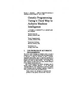
Fig. 8. Example of rule set used in the “Saturday Morning’s Weather” problem. The if part is the antecedent, and the then part is the consequent.

by the rules to the total number of the data in the data set S, i.e., ca(R) = CS(R) / S . The complexity of the rule set R is the number of rules in it, i.e., R . A sample s can fire several rules in the rule set, and their consequents could be contradictory, predicting different classes. In this case, s is assigned the class predicted by the rule of the highest ca, i.e., s.c = r.consequent, where r = arg maxri ∈R ca(ri ), and ri ∈ R is one of the rules fired by s. Fig. 8 gives an example of the rule set used in the “Saturday Morning’s Weather” problem. The problem has four predictive attributes and one binary class attribute. The if part is the antecedent, and the then part is the consequent. While IMGP extracts program trees from the IM, CMRL extracts rules from CM. As the name implies, CM is composed of cells of conditions. The fitness of a condition is used as the criterion to determine whether it is selected as a part of a rule. Information entropy (IE) [16] is frequently used in DTs [13] because it measures how well an attribute classifies the data. CMRL uses IE as the fitness of a condition to measure the degree to which the condition classifies the data. Equation (8) computes the IE of a condition con, with respect to the current data, where p(ci |con) is the conditional probability of the class ci , given the condition con. The conditional probability is calculated based on the data matching the conditions already extracted in the antecedent, so it may change if the previously extracted conditions change. We have iecon = −

m


p(ci |con) log2 p(ci |con).

(8)

i=1

CM has fixed numbers of rows and columns. An attribute can appear only once in a rule; otherwise, multiple conditions of the same attribute would be either redundant or contradictory. Therefore, the height of CM is the number of attributes, i.e., m + 1. Because CMRL uses the entropy of a condition as its fitness, and multiple copies of the same condition would have the same entropy, each row of CM has a single copy of a type of condition. The width of CM is therefore the number of all possible conditions, i.e., ni=1 qi + k. Table IX shows the CM of “Saturday Morning’s Weather” problem, which has four predictive attributes and one binary class attribute.

LI et al.: INSTRUCTION-MATRIX-BASED GENETIC PROGRAMMING

1047

TABLE IX CMOF SATURDAY MORNING’S WEATHER. EACH CELL IS A CONDITION THAT ASSIGNS A VALUE TO AN ATTRIBUTE

2) Algorithm: The overall algorithm of CMRL in Algorithm 4 is similar to IMGP. CMRL keeps extracting rules, grouping them into rule sets, and evaluating the classification accuracies of the rule sets. For each rule set, it puts the best rule aside in a separate persistent rule set, whose reduct is output as the optimal rule set. However, there are a few differences from IMGP. Algorithm 4: The Main Program of CMRL Output: the REDUCT of the elitist rule set} initialize CM; Elitist ← ∅; for gen from 0 to G do for num from 0 to P do R ← ∅; CA ← inf ; while ca(R) < CA do CA ← ca(R); extract a rule r from CM; R ← R ∪ {r}; ca(R) ← evaluate(R); end r ← best ∈ R; if ca(r ∪ Elitist) > ca(Elitist) then Elitist ← Elitist ∪ r; end end REDU CT ← reduct(Elitist)

Extraction: CMRL keeps extracting rules from CM until the rule set of the extracted rules satisfies a predefined classification accuracy. To extract a rule, it starts extracting the first condition from the first row of CM and continues to extract other possible conditions from the following rows until a condition of the class attribute is extracted. The conditions extracted before the class attribute constitute the antecedent of the rule, and the condition of the class attribute is the consequent of the rule. To extract a condition, CMRL randomly selects two conditions on the same row, compares their entropies, and extracts the one with lower entropy. Note that the entropy is not stored with the condition, because the entropy is calculated online with respect to the data matching the conditions already extracted. Elitism: In a rule set, the best rule achieves the highest penalized classification accuracy among all the rules. Such a rule is called an elitist, and it should be reserved in a separate elitist rule set for future use. Before it is put in the elitist rule set, it is checked whether it correctly classifies some data that the other elitist rules classify incorrectly. If not, the best rule is not reserved. The checking avoids keeping redundant rules unnecessarily and reduces the number of elitist rules

TABLE X COMPARISON OF THE RESULTS OF CMRL WITH AND W ITHOUT R ULE -R EDUCT

significantly. While all the extracted rule sets are discarded after evaluation, their best rules are reserved in the elitist rule set. At the end of evolution, the elitist rule set is output for further processing of reduct. Rule-reduct: According to the theory of Occam’s razor, the more complex the model is, the worse the model generalizes. Therefore, not only does the large rule set causes long classification time, but it also may not perform well on the testing data. To reduce the size of the elitist rule set without sacrificing its classification accuracy, we introduce rule-reduct as in Definition 5.1. A rule set can have more than one rulereduct, but we are most interested in the smallest size rulereduct because its generalization is likely to be the best. Definition 5.1: The rule set R is the rule-reduct of the rule set R if and only if ca(R ) = ca(R) and for any R ⊂ R , ca(R ) ≤ ca(R ). After evolution, CMRL uses a greedy approach to find a small rule-reduct of the elitist rule set. CMRL selects the rules from the elitist rule set one after another in the descending order of their classification accuracies and puts them in an initially empty rule set. CMRL stops selecting rules when the classification accuracy of the new rule set is equal to that of the original elitist rule set. This new rule set is thus the rulereduct of the original elitist rule set. Because the rules of high classification accuracies are selected first, the new rule set is likely to be the smallest rule-reduct. 3) Result: To evaluate the performance of CMRL on classification problems, we applied it to four classification problems from the UCI repository [4]. Pima and Horse are the binary class problems already tested by IMGP. Flare has six classes, and Zoo has seven classes. Table X reports the average results over ten runs, where classification error is the ratio of the number of the data misclassified to the size of the whole data set. It also compares the testing errors and the sizes of the rule sets with or without reduct. The generalization of CMRL was acceptable. Except for the Flare problem, the testing errors are only slightly larger than the training errors. The testing error on Pima is even better than that of IMGP, and the testing error on Horse is also better than those of G3 P. Our experiments also show that the differences between the testing errors with or without reduct are only marginal. This implies that reduct does not affect the generalization.

1048

IEEE TRANSACTIONS ON SYSTEMS, MAN, AND CYBERNETICS—PART B: CYBERNETICS, VOL. 38, NO. 4, AUGUST 2008

However, the number of rules in the rule set is decreased significantly, and thus, reduct has saved a lot of computation time in testing. VI. C ONCLUSION We have proposed a new IMGP paradigm. It maintains an IM to store the fitness of the instructions and the links between the instructions and their best subtrees. IMGP extracts program trees from the IM, updates the IM with the fitness of the extracted program trees, performs crossover and mutation on the extracted program trees, and shuffles the IM to propagate good instructions. The experimental results have verified its effectiveness and efficiency on the benchmark problems. It is not only superior to CGP in terms of the qualities of the solutions and the number of program evaluations, but it also outperforms the related GP algorithms on the tested problems. The reason behind why IMGP works can be explained in three perspectives. First, by evolving instructions separately, IMGP actually decomposes a high-dimensional problem into small problems of only one dimension. Therefore, both the size of the solution space and the search time is reduced significantly. At the same time, it also maintains the interdependencies between instructions in the form of the links of best subtrees, and thus, it is likely that the combination of the optimal instructions is the optimal program tree to the original problem. Second, IMGP can be viewed as evolving schemata directly [22]. The schema theory originally explained why GA works. It was extended to explain the mechanism of GP later. By maintaining the average and the best fitness of the instructions and the subtrees, IMGP is able to maintain most of the information of the schemata and to make use of the information to evolve schemata directly. Third, from the cooperative coevolution perspective, the IM is a set of subpopulations of instructions and subtrees. The selected instructions or subtrees from the subpopulations cooperate to form a complete program tree. While the fitness of the tree nodes and the subtrees is evaluated as a whole, they evolve on their own. IMGP can also be used for classification problems. To enhance its performance, IMGP uses gradient descent to find the optimal constants in program trees and incorporates the penalty of program tree complexity in the fitness. In most of the tested problems, IMGP is able to find classifiers of higher classification accuracies than four other GP classifiers. The results of IMGP are also comparable to or better than those of a DT, a neural network, and an SVM. IMGP has a flexible architecture. To solve multiclass classification problems, we have extended IMGP to CMRL. CMRL extracts rules from a CM and groups them as a rule set. The rule-reduct decreases the number of rules in the elitist rule set while maintaining its classification accuracy. In the experiments, CMRL finds effective classifiers on the two multiclass classification problems. For the two binary classification problems, it is also comparable to other GP-based binary classifiers with respect to the testing error.

ACKNOWLEDGMENT The authors would like to thank the anonymous reviewers for their valuable comments and suggestions.

R EFERENCES [1] W. Banzhaf, P. Nordin, R. E. Keller, and F. D. Francone, Genetic Programming—An Introduction: On the Automatic Evolution of Computer Programs and Its Applications. San Mateo, CA: Morgan Kaufmann, Jan. 1998. [2] F. H. Bennett, III, J. R. Koza, J. Shipman, and O. Stiffelman, “Building a parallel computer system for $18,000 that performs a half peta-flop per day,” in Proc. GECCO, W. Banzhaf, J. Daida, A. E. Eiben, M. H. Garzon, V. Honavar, M. Jakiela, and R. E. Smith, Eds., San Francisco, CA, 1999, pp. 1484–1490. [3] C. M. Bishop, Neural Networks for Pattern Recognition. Oxford, U.K.: Clarendon, 1995. [4] E. K. C. Blake and C. J. Merz, UCI Repository of Machine Learning Databases, 1998. [Online]. Available: http://www.ics.uci.edu/~mlearn/ MLRepository.html [5] E. Bonabeau, M. Dorigo, and G. Theraulaz, Swarm Intelligence: From Natural to Artificial Systems. New York: Oxford Univ. Press, 1999. [6] P. A. N. Bosman and E. D. de Jong, “Grammar transformations in an EDA for genetic programming,” in Proc. GECCO Workshop, Seattle, WA, Jun. 2004. [7] E. Burke, S. Gustafson, and G. Kendall, “Diversity in genetic programming: An analysis of measures and correlation with fitness,” IEEE Trans. Evol. Comput., vol. 8, no. 1, pp. 47–62, Feb. 2004. [8] C. Cortes and V. Vapnik, “Support-vector networks,” Mach. Learn., vol. 20, no. 3, pp. 273–297, Sep. 1995. [9] I. Dempsey, M. O’Neill, and A. Brabazon, “Constant creation in grammatical evolution,” Int. J. Innov. Comput. Appl., vol. 1, no. 1, pp. 23–38, Apr. 2007. [10] P. D’haeseleer, “Context preserving crossover in genetic programming,” in Proc. IEEE World Congr. Comput. Intell., Orlando, FL. Piscataway, NJ: IEEE Press, Jun. 1994, vol. 1, pp. 256–261. [11] M. Dorigo, V. Maniezzo, and A. Colorni, “Ant system: Optimization by a colony of cooperating agents,” IEEE Trans. Syst., Man Cybern. B, Cybern., vol. 26, no. 1, pp. 29–41, Feb. 1996. [12] J. Eggermont, A. E. Eiben, and J. I. van Hemert, “A comparison of genetic programming variants for data classification,” in Proc. 11th BNAIC, E. Postma and M. Gyssens, Eds., Maastricht, The Netherlands, Nov. 1999, pp. 253–254. [13] R.-E. Fan, P.-H. Chen, and C.-J. Lin, “Working set selection using second order information for training support vector machines,” J. Mach. Learn. Res., vol. 6, pp. 1889–1918, Dec. 2005. [14] C. Ferreira, “Gene expression programming: A new adaptive algorithm for solving problems,” Complex Syst., vol. 13, no. 2, pp. 87–129, Feb. 2001. [15] D. E. Goldberg, Genetic Algorithms in Search, Optimization & Machine Learning. Reading, MA: Addison-Wesley, 1989. [16] R. M. Gray, Entropy and Information Theory. New York: SpringerVerlag, 1990. [17] G. Harik, “Linkage learning via probabilistic modeling in the ECGA,” Univ. Illinois Urbana-Champaign, Urbana, IL, Tech. Rep. IlliGAL No. 99 010, 1999. [18] T. Hastie, R. Tibshirani, and J. H. Friedman, The Elements of Statistical Learning. New York: Springer-Verlag, Jul. 2001. [19] J. R. Koza, Genetic Programming: On the Programming of Computers by Natural Selection. Cambridge, MA: MIT Press, 1992. [20] J. R. Koza, Genetic Programming—Part II: Automatic Discovery of Reusable Programs. Cambridge, MA: MIT Press, May 1994. [21] K. S. Leung, K. H. Lee, and S. M. Cheang, “Parallel programs are more evolvable than sequential programs,” in Proc. 6th EuroGP, Essex, U.K., E. C. C. Ryan, T. Soule, M. Keijzer, E. Tsang, and R. Poli, Eds. New York: Springer-Verlag, 2003, vol. 2610, pp. 107–118. [22] G. Li, K.-H. Lee, and K.-S. Leung, “Evolve schema directly using instruction matrix based genetic programming,” in Proc. 8th Eur. Conf. Genetic Program., Lausanne, Switzerland, M. Keijzer, A. Tettamanzi, P. Collet, J. I. van Hemert, and M. Tomassini, Eds. New York: Springer-Verlag, Mar. 2005, vol. 3447, pp. 271–280. [23] T. Loveard and V. Ciesielski, “Representing classification problems in genetic programming,” in Proc. Congr. Evol. Comput., COEX, Seoul, Korea. Piscataway, NJ: IEEE Press, May 2001, vol. 2, pp. 1070–1077. [24] D. MacKay, Information Theory, Inference, and Learning Algorithms, Sep. 2003. [25] J. F. Miller and P. Thomson, “Cartesian genetic programming,” in Proc. 3rd EuroGP, Edinburgh, U.K., R. Poli, W. Banzhaf, W. B. Langdon, J. Miller, P. Nordin, and T. C. Fogarty, Eds. New York: Springer-Verlag, 2000, vol. 1802, pp. 121–132.

LI et al.: INSTRUCTION-MATRIX-BASED GENETIC PROGRAMMING

[26] D. J. Montana, “Strongly typed genetic programming,” Evol. Comput., vol. 3, no. 2, pp. 199–230, 1995. [27] T. Perkis, “Stack-based genetic programming,” in Proc. IEEE World Congr. Comput. Intell., Orlando, FL. Piscataway, NJ: IEEE Press, Jun. 1994, vol. 1, pp. 148–153. [28] R. Poli, “Evolution of graph-like programs with parallel distributed genetic programming,” in Proc. 7th ICGA, T. B¨ack, Ed., 1997, pp. 346–353. [29] M. Potter and K. De Jong, “Cooperative coevolution: An architecture for evolving coadapted subcomponents,” Evol. Comput., vol. 8, no. 1, pp. 1– 29, Mar. 2000. [30] J. Quinlan, Data Mining Tools See5 and C5.0, 2007. [Online]. Available: http://www.rulequest.com/see5-info.html [31] R. Quinlan, “Induction of decision trees,” Mach. Learn., vol. 1, no. 1, pp. 81–106, 1986. [32] S. A. Rojas and P. J. Bentley, “A grid-based ant colony system for automatic program synthesis,” in Proc. Genetic Evol. Comput. Conf., M Keijzer, Ed., Seattle, WA, Jul. 2004. Late Breaking Papers. [33] R. Salustowicz and J. Schmidhuber, “Probabilistic incremental program evolution,” Evol. Comput., vol. 5, no. 2, pp. 123–141, 1997. [34] K. Sastry and D. E. Goldberg, “Probabilistic model building and competent genetic programming,” in Genetic Programming Theory and Practice, R. L. Riolo and B. Worzel, Eds. Norwell, MA: Kluwer, 2003, ch. 13, pp. 205–220. [35] Y. Shan, R. I. McKay, H. A. Abbass, and D. Essam, “Program evolution with explicit learning: A new framework for program automatic synthesis,” in Proc. CEC, R. Sarker, R. Reynolds, H. Abbass, K. C. Tan, B. McKay, D. Essam, and T. Gedeon, Eds., Canberra, Australia, Dec. 2003, pp. 1639–1646. [36] Y. Shan, R. I. McKay, R. Baxter, H. Abbass, D. Essam, and H. Nguyen, “Grammar model-based program evolution,” in Proc. IEEE Congr. Evol. Comput., Portland, OR, Jun. 20–23, 2004, pp. 478–485. [37] D. Thierens and D. E. Goldberg, “Mixing in genetic algorithms,” in Proc. 5th Int. Conf. Genetic Algorithms, S. Forrest, Ed., San Mateo, CA, 1993, pp. 38–45. [38] A. Tsakonas, “A comparison of classification accuracy of four genetic programming-evolved intelligent structures,” Inf. Sci., vol. 176, no. 6, pp. 691–724, Mar. 2006. [39] J. F. Wang, K. H. Lee, and K. S. Leung, “Condition matrix based genetic programming for rule learning,” in Proc. 18th IEEE ICTAI, Washington, DC, Nov. 2006, pp. 315–322. [40] P. A. Whigham, “Grammatically-based genetic programming,” in Proc. Workshop Genetic Program: From Theory Real-World Appl., J. Rosca, Ed., San Mateo, CA, Jul. 1995, pp. 33–41. [41] M. L. Wong and K. S. Leung, “Data mining using grammar based genetic programming and applications,” in Genetic Programming, vol. 3. Norwell, MA: Kluwer, Jan. 2000. [42] K. Yanai and H. Iba, “Estimation of distribution programming based on Bayesian network,” in Proc. CEC, R. Sarker, R. Reynolds, H. Abbass, K. C. Tan, B. McKay, D. Essam, and T. Gedeon, Eds., Canberra, Australia, Dec. 2003, pp. 1618–1625. [43] M. Zhang and W. Smart, “Genetic programming with gradient descent search for multiclass object classification,” in Proc. 7th EuroGP, Coimbra, Portugal, M. Keijzer, U.-M. O’Reilly, S. M. Lucas, E. Costa, and T. Soule, Eds. New York: Springer-Verlag, Apr. 2004, vol. 3003, pp. 399–408. [44] D. Zongker and B. Punch, “lilgp 1.01 User’s Manual,” Michigan State Univ., East Lansing, MI, Tech. Rep., Mar. 1996.

Gang Li (S’07) was born in China in 1979. He received the B.E. degree in computer science from Wuhan University, Wuhan, China, in 2002. He is currently working toward the Ph.D. degree at The Chinese University of Hong Kong, Shatin. His current research interests include evolutionary computation, independent component analysis, and bioinformatics.

1049

Jin Feng Wang was born in Hebei, China, in 1978. She received the B.S. degree in computer science from the Hebei Science and Technology University, Hebei, China, in 1999, and the M.S. degree in computer science from Hebei University in 2003. She is currently working toward the Ph.D. degree at the Department of Computer Science and Engineering, The Chinese University of Hong Kong, Shatin.

Kin Hong Lee (SM’90) received the B.Sc. and M.Sc. degrees in computer science from the University of Manchester, Manchester, U.K. Prior to joining the Chinese University of Hong Kong, Shatin, in 1984, he had worked for Burroughs Machines, Cumbernauld, U.K., and International Computers, Ltd., Manchester. He is currently an Associate Professor with the Department of Computer Science and Engineering, The Chinese University of Hong Kong, Shatin. His current interests are computer hardware and bioinformatics. He has over 60 published papers in these fields.

Kwong-Sak Leung (M’77–SM’89) received the B.Sc. degree in electronic engineering and the Ph.D. degree in 1977 and 1980, respectively, from the University of London, London, U.K. He was a Senior Engineer on contract R&D with ERA Technology. He later joined the Central Electricity Generating Board to work on nuclear power station simulators in the U.K. He joined the Department of Computer Science and Engineering, The Chinese University of Hong Kong, Shatin, in 1985, where he is currently a Professor of computer science and engineering. He is on the Editorial Board of Fuzzy Sets and Systems and is an Associate Editor for the International Journal of Intelligent Automation and Soft Computing. His research interests are in soft computing and bioinformatics, including evolutionary computation, parallel computation, probabilistic search, information fusion and data mining, and fuzzy data and knowledge engineering. He has authored and coauthored over 200 papers and two books in fuzzy logic and evolutionary computation. Dr. Leung is a Chartered Engineer, a member of the Institution of Engineering and Technology and the Association for Computing Machinery, a Fellow of the Hong Kong Institution of Engineers, and a Distinguished Fellow of the Hong Kong Computer Society. He has been the Chair and a member of many program and organizing committees of international conferences.