Integer goal programming approach for finding a compromise ...

MultiCraft

INTERNATIONAL JOURNAL OF ENGINEERING, SCIENCE AND TECHNOLOGY www.ijest-ng.com

International Journal of Engineering, Science and Technology Vol. 3, No. 6, 2011, pp. 184-195

© 2011 MultiCraft Limited. All rights reserved

Integer goal programming approach for finding a compromise allocation of repairable components Irfan Ali*, Yashpal Singh Raghav and Abdul Bari Department of Statistics and Operations Research Aligarh Muslim University, Aligarh, INDIA *Corresponding author email id: [email protected]

Abstract The selection problem of repairable components for a system is a kind of reliability optimization problem and is often treated as a single objective problem with the goal of maximizing the system reliability (or minimizing either time or cost spent on repairing the component). In the present paper, we formulated the selection problem of repairable components for a parallelseries system as a multi-objective optimization problem and have discussed two different models. In the first model, the reliability of subsystems are considered as different objectives. In second model the cost and time spent on repairing the components are considered as two different objectives. Selective maintenance operation is used to select the repairable components and a multi-objective goal programming algorithm is proposed to obtain compromise selection of repairable components for the two models under some given constraints. A numerical example is given to illustrate the procedure. Keywords: Reliability, Goal Programming, Compromise allocation, Multi-objective programming. DOI: http://dx.doi.org/10.4314/ijest.v3i6.15 1. Introduction Every industrial and engineering organization recognizes that the maintenance can provide value to their organization. The production losses occur due to system failure and therefore, industries try to seek more efficient and effective maintenance policy. Industrial organizations recognize that effective maintenance policies can improve their production. In most maintenance optimization models, only maintenance cost factor is taken into account and maintenance action duration (repairing and replacing times) is assumed to be negligible (Pham and Wang 1996). However, making the above assumptions can have a big influence on the determination of the optimal maintenance policy. The maintenance action duration and the cost are important factors to take into account in the maintenance optimization process because practically the maintained component is not always restored as good as new one. All maintenance optimization models start from a certain maintenance policy and try to optimize this specific policy. The output of the optimization model also depends on the maintenance policy and actions used. For example, a time-based maintenance policy will optimize the timing of maintenance, while a condition-based maintenance policy also tries to optimize the time of inspection. In most of the maintenance optimization models the objective function takes into account only one criteria (e.g., cost, availability, reliability, time). This makes these models only single-objective but when we look to real-life problems a multi-objective optimization is required. This paper presents a new contribution in the field of system reliability optimization for compromise selection problem of repairable components. A multi-objective goal programming algorithm is proposed to obtain compromise selection of repairable components. The use of goal programming allows considering multiple criteria to achieve the goals and satisfy the constraints and the lexicographic goal programming technique allows the analyst to assign different priorities to the goals considered, looking for a solution that first of all meets the most important of these priorities. Goal programming, introduced by Charnes and Cooper (1961), deals with the problem of achieving a set of conflicting goals. The objective function searches to minimize deviations from the set of pre-assigned goals. It has been studied by many researchers

Ali et al. / International Journal of Engineering, Science and Technology, Vol. 3, No. 6, 2011, pp. 184-195

185

El-Sayed et al. (1989), Schniederjans et al. (1982), (1989), Lin (1980), Kvanil (1980) and Taylor et al. (1982) etc. and successfully applied to many diverse, real life problems, such as production planning, financial decisions, marketing decisions, corporate planning, academic planning, and decision in government sectors etc. Lexicographic goal programming is a special case of goal programming, in which the most important (upper level) goals are optimized before least important goals. The idea of applying lexicographic goal programming comes from its solution structures, in which it works with more than one objective at a time. Coit et al. (2004) proposed a multiple objective formulation where the objectives were to maximize an estimate of the system reliability and to minimize the variance of that estimate. Coit and Konak (2006) proposed a new heuristic technique for system reliability optimization. The selective maintenance operation is an optimal decision-making activity for systems consisting of several components under limited maintenance duration. The main objective of the selective maintenance operation is to select the most important component in subsystem. Rice et al. (1998) were the first to deal with the selective maintenance problem. Lust et al. (2009) also proposed a selective maintenance optimal model for the general series–parallel system containing multiple components to maximize system reliability after the maintenance action, and presented a solution algorithm by integrating the heuristic method with tabu search (TS). Ali et al. (2011a, b) considered the problem of optimum allocation of repairable and replaceable components for seriesparallel system by using selective maintenance. In this paper, we formulate the problem of repairable components for a parallel-series system as a multi-objective optimization problem. The two different models are discussed. In the first model, the reliability of subsystems is considered as different objectives of maximizing the system reliability under the limited cost spent and time taken on repairing the components. In the second model the cost and time spent on repairing the components are considered as two different objectives and simultaneously minimizing the cost spent and time taken on repairing the system under the given upper bound on system reliability. The multiobjective NLPPS are solved by “Goal Programming Techniques” using software package LINGO. LINGO is a user’s friendly package for constrained optimization developed by LINDO Systems Inc. A user’s guide- LINGO User’s Guide (2001) is also available. For more information one can visit the site http://www.lindo.com. 2. Statement of the problem and notations In every industry, systems are used in the production of goods. If such systems deteriorate or fail, the effect can be wide spread. Indeed, system deterioration is often reflected in higher production cost, time, lower product quality and also quantity. The system maintenance decision is taken on the basis of the state condition of the system (i.e. whether the system is good or bad). The aim is to present a model of reliability improvement maintenance policies that minimizes the total cost and time spent on maintaining a system. For this purpose, we consider a system which requires performing a sequence of identical production runs after every given (fixed) period. The system consists of several subsystems where each subsystem can work properly if at least one of its components is operational. For the given problem, the following assumptions have been made: (i) all components states are independent (ii) reliability, cost and time of each component in one subsystem are same (iii) each constraint is an increasing function of d i . Let ri denotes the probability that a component of a subsystem i survives the production runs given that the component is functioning at the start of the production runs, and let ni denotes the number of components in subsystem i which are in operational state at the start of the production run. The following notations are used in the problem: R: T0 : C0 :

Reliability of the system Total available repair time for the system Total available repair cost for the system Reliability of each component available for subsystem

i

ri

:

ti

: Repair time of each component available for subsystem i

ni m

θi βi ci ai

: : : : : :

Maximal number of components in each subsystem i Number of subsystems Parameters associated with the time of components in subsystem i Parameters associated with the cost of components in subsystem i Cost of each component available for subsystem i Total number of failed components in subsystem i


186

di

:

The number of components in subsystem i repaired prior to the next production runs

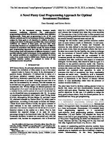
Fig.1 illustrate a system which is a series arrangement of the subsystems (subsystem1, subsystem 2… subsystem m), with reliability as

∏ {1 − (1 − r ) } m

R=

ni

i

(1)

i =1

At the completion of particular production runs, each component in the system is either functioning or failed. Ideally all the failed components in the subsystems are repaired and then replaced back prior to the beginning of the next production runs. However, due to the constraints on the time and cost, it may not be possible to repair all the failed components in the system. The time required for repairing and then replacing back all the failed components in the system is given by m

∑t

T =

i

(2)

ai

i =1

The maintenance time available for repairing and then replacing back the failed components between two production runs is T0 units. If T0 < T , then all failed components can not be repaired and then replaced back prior to beginning of the next production run. The cost required for replacing the failed components after repairs in the system is given by m

C=

∑c

i

(3)

ai

i =1

The maintenance cost available for repairing and then replacing back the failed components between two production runs is C 0 units. If C 0 < C , then all failed components can not be repaired and replaced back prior to beginning of the next production run. In such cases, a method is needed to decide which failed components should be repaired and replaced back prior to the next production run and the rest be left in a failed condition. This process is referred as selective maintenance (See Rice et al., 1998). In th

the selective maintenance the number of components available for the next production run in the i subsystem will be (ni − a i ) + d i , i = 1, 2, ..., m The reliability of the given system is defined as

∏ {1 − (1 − r ) m

R =

i

ni − ai + d i

}

(4)

(5)

i =1

The repair time constraint for the system is given as m

∑ t [d i

i

+ exp(θ i d i )] ≤ T0

(6)

i =1

where exp(θ i d i ) is the additional time spent due to the interconnection between parallel components. The repair cost constraint for the system is defined as m

∑ c [d i

i

+ exp( β i d i )] ≤ C 0

(7)

i =1

where exp( β i d i ) is the additional cost amount due to the interconnection between parallel components.


187

3. Multi-Objective Optimal Maintenance Problem on Parallel-Series System Model 1: The reliability of the system can be maximized if we maximize the reliability of each individual subsystem. This is a logical approach as system reliability is the product of the subsystem reliabilities so if they are maximized, the system reliability will also be maximized. The mathematical model of the problem is given as: Maximize (R1 , R 2 , K R m ) ⎫ ⎪ ⎪ ⎪ subject to ⎪ m ⎪⎪ t i [d i + exp(θ i d i )] ≤ T0 (8) ⎬ i =1 ⎪ m ⎪ ⎪ c i [d i + exp( β i d i )] ≤ C 0 ⎪ i =1 ⎪ and 0 ≤ d i ≤ a i , i = 1,2,..., m and integers ⎭⎪

∑

∑

{

}

where Ri = 1 − (1 − ri ) ni − ai + d i , i = 1, 2, ..., m. Model 2: Here we have formulated a multi-objective programming problem in which time and the cost spent on system maintenance are minimized simultaneously for the required reliability R * (say). The mathematical model of the problem is given as: m ⎫ Min C = c i [d i + exp(β i d i )] ⎪ ⎪ i =1 ⎪ and ⎪ m ⎪ ⎪⎪ Min T = t i [d i + exp(θ i d i )] (9) ⎬ i =1 ⎪ subject to ⎪ m ⎪ ⎪ 1 − (1 − ri )ni − ai + d i ≥ R * ⎪ i =1 ⎪ and 0 ≤ d i ≤ a i , i = 1,2,..., m and integers⎭⎪

∑

∑

∏

4. Methods of Solution Method 1: The Goal Programming Approach Model 1: We use goal programming technique to solve problem (8). For this purpose, we first solve the following m Non Linear Programming Problems (NLPPs) for all the ‘m’ subsystems separately.

{

}

⎫ ⎪ ⎪ ⎪ subject to ⎪ m ⎪⎪ t i [d i + exp(θ i d i )] ≤ T0 ⎬ i =1 ⎪ ⎪ m ⎪ c i [d i + exp( β i d i )] ≤ C 0 ⎪ i =1 ⎪ 0 ≤ d i ≤ a i , i = 1,2,..., m and integers ⎪⎭

Maximize Ri = 1 − (1 − ri ) ni − ai + d i

∑

i = 1,2,..., m

(10)

∑

and

(

)

Let d ∗i = d i∗1 , d i∗2 , . . ., d i∗ m denote the solution to the i-th NLPP in (10) with Ri∗ as the value of the objective function given by

R = {1 − (1 − ri ) ∗ i

Further, let

d ∗c

=

(

ni − ai + d i

}, i = 1, 2, ..., m. ) be the vector of optimum compromise allocations with

d 1∗c , d 2∗ c , . . ., d m∗ c

(11)


188

{

Ri∗c = 1 − (1 − ri )

ni − ai + d i c

} as the optimal value of the objective function for i-th subsystems under this allocation.

Obviously, Ri∗c ≤ Ri∗ or Ri∗c − Ri∗ ≤ 0 ;

i = 1,2, . . ., m.

(12)

A reasonable criterion to work out a compromise allocation is to minimize the sum of deviations between the reliabilities i.e. δ i = R ∗i − Ri∗c .

(

)

Now the multi-objective NLPP can be formulated as a single objective NLPP m ⎫ Minimize δi ⎪ ⎪ i =1 ⎪ subject to ⎪ Ri*c + δ i = Ri* , i = 1, ... , m ⎪ ⎪ m ⎪⎪ t i [d i + exp(θ i d i )] ≤ T0 ⎬ ⎪ i =1 ⎪ m ⎪ c i [d i + exp( β i d i )] ≤ C 0 ⎪ i =1 ⎪ ⎪ δ i ≥ 0, i = 1, ... , m ⎪ and 0 ≤ d i ≤ a i , i = 1,2,..., m and integers ⎪ ⎭

∑

∑

(13)

∑

(

)

where d ∗c = d 1∗c , d 2∗ c , . . ., d m∗ c denotes a compromise allocation with reliabilities

{

Ri c = 1 − (1 − ri )

ni − ai + d i c

}, i = 1, 2, ..., m

(14)

and δ i ≥ 0; i = 1,2, . . ., m are called goal variables whose values are to be determined.

(

)

The goal is to find the compromise allocation d ∗c = d 1∗c , d 2∗ c , . . ., d m∗ c such that the deviations in the i-th subsystem reliability due to the use of compromise allocation should not exceed δ i ; i = 1,2, . . ., m and

m

∑δ

i

is minimum.

i =1

NLPP (13) may be restated as: ⎫ ⎪ ⎪ i =1 ⎪ subject to ⎪ ⎪ 1 − (1 − ri ) ni − ai + d i + δ i = Ri* , i = 1, ... , m ⎪ m ⎪⎪ t i [d i + exp(θ i d i )] ≤ T0 ⎬ ⎪ i =1 ⎪ m ⎪ c i [d i + exp( β i d i )] ≤ C 0 ⎪ i =1 ⎪ ⎪ δ i ≥ 0, i = 1, ... , m ⎪ and 0 ≤ d i ≤ a i , i = 1,2,..., m and integers ⎭⎪ m

Minimize

{

∑δ

i

}

∑

(15)

∑

where the value of Ri c is substituted from (14) and the compromise allocation d i c , i = 1,2, . . . , m is replaced by d i for simplicity. The optimal solution to the NLPP (15) will be the required optimum compromise allocation d ∗c that minimizes the sum of deviations of the reliabilities from their optimum values. Model 2: As discussed in model 1, to solve the problem (9) using goal programming, we first solve the following Non Linear Programming Problems (NLPPs) to minimize repair time and cost with respect to predetermined reliability requirement for all the ‘m’ subsystems separately.


189

m

Min. T =

∑t

i

[d i + exp(θ i d i )]

i =1

subject to m

∏ 1 − (1 − r ) i

ni − ai + d i

≥R

*

i =1

0 ≤ d i ≤ a i , i = 1,2, ... , m

⎫ ⎪ ⎪ ⎪ ⎪ ⎬ ⎪ ⎪ ⎪ ⎪⎭

(16)

⎫ ⎪ ⎪ ⎪ ⎪ ⎬ ⎪ ⎪ ⎪ ⎪⎭

(17)

and m

Min. C =

∑C

i

[d i + exp(β i d i )]

i =1

subject to m

∏ 1 − (1 − r ) i

ni − ai + d i

≥R

*

i =1

0 ≤ d i ≤ a i , i = 1,2, ... , m

(

)

Let d ∗j = d ∗j 1 , d ∗j 2 , . . ., d ∗j m , j = 1, 2 denote the solution to the NLPP (16) and (17) with T0∗ and C 0∗ as the value of the objective functions given by m

T0* =

∑t

[d i + exp(θ i d i )]

i

(18)

i =1 m

C 0* =

∑C = (d

i


i =1

Further, let d ∗c

∑ [ m

T0*c =

∗ ∗ ∗ 1 c , d 2 c , . . ., d m c

(

t i d i + exp θ i d i c

)] and

(19)

) be the vector of optimum compromise allocations with ∑ C [d m

C 0* c =

i =1

i

i

(

+ exp β i d i c

)]

as the optimal value of the objective functions for the NLPP

i =1

(16) & (17) under this allocation. Obviously, T0∗c ≥ T0∗ or T0∗c − T0∗ ≥ 0 and

C 0∗c ≥ C 0∗ or

C 0∗c − C 0∗ ≥ 0

(20) (21)

A reasonable criterion to workout a compromise allocation is “Minimizing the sum of deviations in the repair time and cost due to the use of the compromise allocation”. We may express the NLPP (16) and (17) using (20) and (21) with the above compromise criterion as the following single objective NLPP 2 ⎫ δj Minimize ⎪ ⎪ j =1 ⎪ subject to ⎪ ⎪ * * To c − δ 1 = T0 ⎪ ⎪ * * (22) Co c − δ 2 = C0 ⎬ ⎪ m ⎪ 1 − (1 − ri )ni − ai + d i ≥ R * ⎪ i =1 ⎪ ⎪ δ j ≥ 0, j = 1, 2 ⎪ and 0 ≤ d i ≤ a i , i = 1,2,..., m and integers⎪ ⎭

∑

∏

(

)

where d ∗c = d 1∗c , d 2∗ c , . . ., d m∗ c denotes a compromise allocation with repair time and cost

∑ t [d m

T0*c =

i

i =1

i

(

+ exp θ i d i c

)]

(23)


190

∑ C [d m

and

C 0* c =

i

i

(

+ exp β i d i c

)]

(24)

i =1

and δ j ≥ 0;

j = 1, 2 are called goal variables whose values are to be determined.

(

)

The goal is to find the compromise allocation d ∗c = d 1∗c , d 2∗ c , . . ., d m∗ c such that the deviations in the i-th subsystem repair time and cost due to the use of compromise allocation should not exceed δ j ≥ 0, j = 1, 2 and

2

∑δ

j

is minimum. NLPP (22) may be

j =1

restated as: 2

∑δ

Minimize

j

j =1

subject to m

∑ t [d i

i

i =1 m

∑ c [d i

i

+ exp(θ i d i )] − δ 1 = T0* + exp( β i d i )] − δ 2 = C 0*

i =1

m

∏ 1 − (1 − r ) i

ni − ai + d i

≥ R*

i =1

δ j ≥ 0, and

j = 1, 2

0 ≤ d i ≤ a i , i = 1,2,..., m and integers

⎫ ⎪ ⎪ ⎪ ⎪ ⎪ ⎪ ⎪ ⎪ ⎪⎪ ⎬ ⎪ ⎪ ⎪ ⎪ ⎪ ⎪ ⎪ ⎪ ⎪ ⎪⎭

(25)

where the values of T0∗c and C 0∗c are substituted from (23) & (24) and the compromise allocation d i c is replaced by d i for simplicity. The optimal solution to the NLPP (25) will be the required optimum compromise allocation d ∗c that minimizes the sum of deviations of the repair time and cost from their optimum values. NLPP (15) and (25) can be solved by using software package LINGO. In the next section a numerical example is given to illustrate the Goal Programming Approach. Method 2: Lexicographic (Preemptive) Goal Programming Approach Model 1: Lexicographic goal programming is an important mathematical programming method developed to solve the problems with conflicting linear or non-linear objectives as well as constraints. The user is able to provide levels or targets of achievement for each objective and priorities for the order in which goals are to be achieved. It finds an optimal solution that satisfies as many of the goals as possible, in the order of importance. The approach defines different priority levels Pj for the goals of the analysis. The different priority levels reflect the hierarchical relationship between the targets in the objective function arranged in order of decreasing priority (P1>P2>…>Pm). In order to identify the solution to the problem, the highest priority goals and constraints are considered first; if more than one solution is found in the first step, another goal programming problem is formulated which takes into account the second priority level targets. The procedure is repeated until a unique solution is found, gradually considering decreasing priority levels. In the model 1 defined in section 3, if we give the highest priority to the subsystem which has more failed components i.e. Ri 1 , Ri 2 , K Ri G , where i1 , ..., iG is decreasing order of the priorities. The problem (8) using lexicographic goal

(

)

programming is given as


191

⎫ ⎪ ⎪ ⎪ subject to ⎪ m ⎪⎪ t i [d i + exp(θ i d i )] ≤ T0 ⎬ i =1 ⎪ m ⎪ ⎪ c i [d i + exp( β i d i )] ≤ C 0 ⎪ i =1 ⎪ 0 ≤ d i ≤ a i , i = 1,2,..., m and integers ⎭⎪ Maximize Ri1

∑

(26)

∑

and

If the maximum of problem (26) is R1∗ , then in the next stages we must resolve the problem for maximum values R1∗ , .., RG* −1 . Thus, we reach at stage G, where the next problem to be solved is Maximize RiG ⎫ ⎪ subject to ⎪ ⎪ 1 − (1 − ri ) ni − ai + d i ≥ R1* ⎪ M ⎪ ⎪ ni − ai + d i * ≥ RG −1 1 − (1 − ri ) ⎪ (27) ⎬ m ⎪ t i [d i + exp(θ i d i )] ≤ T0 ⎪ i =1 ⎪ m ⎪ ⎪ c i [d i + exp( β i d i )] ≤ C 0 ⎪ i =1 ⎪ and 0 ≤ d i ≤ a i , i = 1,2,..., m and integers ⎭ Thus, the solution obtained in this stage is the optimum solution to the problem.

{

}

{ ∑

}

∑

Model 2: In model 2, defined in section 3; we want to minimize repairable time and cost for a fixed reliability requirement in which minimization of repairable time is most important than cost. If the minimum of the NLPP (16) is T0∗ , then in the next step

we must resolve the following NLPP for optimum repair cost m ⎫ Min. C = c i [d i + exp(β i d i )] ⎪ ⎪ i =1 ⎪ subject to ⎪ m ⎪ ⎪ t i [d i + exp(θ i d i )] ≤ T0* ⎬ ⎪ i =1 ⎪ m ⎪ 1 − (1 − ri )ni − ai + d i ≥ R * ⎪ i =1 ⎪ and 0 ≤ d i ≤ a i , i = 1,2,..., m and integers⎪⎭

∑

∑

∏{

(28)

}

After solving the NLPP (28) we obtain the optimum repair cost C 0* . 5. Numerical Illustration

Consider a system consisting of 5 subsystems. The available time between two production runs for repairing and replacing back the components is 60 time units. Let the given maintenance cost of the system be 90 units. The other parameters for the various subsystems are given in Table 1.


192

Table 1. The parameters for the numerical example Subsystem 1 2 3 4 5 4 4 4 4 4 ni ri

0.9

0.85

0.85

0.80

0.85

ai

3

2

2

2

3

ci

8

7

8

4

6

ti

3

4

3

5

4

θi βi

0.25

0.25

0.25

0.25

0.25

0.25

0.25

0.25

0.25

0.25

Solution by Using Goal Programming Approach Model 1: Using the values given in Table 1 the NLPP (10) and their optimal solutions d ∗i ; i = 1, 2, 3, 5 with the corresponding

values of Ri∗ are listed below. These values are obtained by software LINGO. For i =1 ⎫ Maximize R1 = 1 − (1 − r1 ) n1 − a1 + d1 ⎪ ⎪ ⎪ subject to ⎪ 5 ⎪⎪ t i [d i + exp(θ i d i )] ≤ 60 ⎬ i =1 ⎪ ⎪ 5 ⎪ c i [d i + exp( β i d i )] ≤ 90 ⎪ i =1 ⎪ and 0 ≤ d i ≤ a i , i = 1,2,..., 5 and integers ⎪⎭

{

}

∑

∑

(

)

∗ ∗ ∗ ∗ ∗ The optimum allocation d 1∗ = d 11 , d 12 , d 13 , d 14 , d 15 is ∗ d11

= 3,

∗ d12

= 0,

∗ d13

= 1,

∗ d14

= 0,

∗ d15

= 0. with

R1*

= 0.9999

Similarly for i = 2, 3, 4 & 5 the results are i =2 * ∗ ∗ ∗ ∗ ∗ d 21 = 0, d 22 = 2, d 23 = 1, d 24 = 1, d 25 = 1. with R 2 = 0.9994 i =3 * ∗ ∗ ∗ ∗ ∗ d31 = 0, d32 = 1, d33 = 2, d34 = 1, d35 = 1. with R3 = 0.9994

i =4 * ∗ ∗ ∗ ∗ ∗ d 41 = 1, d 42 = 1, d 43 = 1, d 44 = 2, d 45 = 1. with R 4 = 0.9984

i =5 * ∗ ∗ ∗ ∗ ∗ d51 = 0, d52 = 0, d53 = 0, d54 = 1, d55 = 3. with R5 = 0.9994

Using the computed values of Ri∗ ; i = 1, 2, 3, 4,5 and the compromise criterion conjectured in section 4 for model 1, the Goal Programming Problem given in (15) may be expressed as:


193

δ1 + δ 2 + δ 3 + δ 4 + δ 5

⎫ ⎪ ⎪ ⎪ subject to ⎪ 1 − ( 1 − r1 ) n1 − a1 + d1 + δ 1 = 0.9999 ⎪ ⎪ n2 − a 2 + d 2 + δ 2 = 0.9994 1 − ( 1 − r2 ) ⎪ ⎪ n3 − a3 + d 3 + δ 3 = 0.9994 1 − ( 1 − r3 ) ⎪ ⎪ 1 − ( 1 − r4 ) n4 − a4 + d 4 + δ 4 = 0.9984 ⎪ (29) ⎬ n5 − a5 + d 5 + δ 5 = 0.9994 1 − ( 1 − r5 ) ⎪ ⎪ m ⎪ t i [d i + exp( θ i d i )] ≤ T0 ⎪ i =1 ⎪ m ⎪ ⎪ c i [d i + exp( β i d i )] ≤ C 0 ⎪ i =1 ⎪ δ i ≥ 0 , i = 1, ... , 5 ⎪ and 0 ≤ d i ≤ a i , i = 1,2,..., m and integers ⎪⎭ The optimum compromise allocation which is the solution to the NLPP (29) given by the optimization software LINGO is: Minimize

{ { { { {

} } } } }

∑

∑

d1∗C = 1, d 2∗C = 1, d3∗C = 1, d 4∗C = 2, d5∗C = 2.

The reliabilities of the subsystems Ri under compromise allocations denoted by ( Ri ) comp. are: ( R1 ) comp. = 0.9900 , ( R 2 ) comp. = 0.9966 , ( R3 ) comp. = 0.9966 , ( R 4 ) comp. = 0.9984 and ( R5 ) comp. = 0.9966 with decreases in the

reliability for the individual subsystems as: δ 1 = 0.0099, δ 2 = 0.0028, δ 3 = 0.0028, δ 4 = 0 and δ 5 = 0.0028 . Model 2: Using the values given in Table 1 the NLPP (16) and (17) for the desired reliability requirement R * ≥ 0.99 has been solved. And optimum allocations for the corresponding values of T0∗ and C 0* are given below for j =1 * ∗ ∗ ∗ ∗ ∗ d11 = 2, d12 = 1, d13 = 2, d14 = 2, d15 = 2 with T0 = 63.90

and j =2 * ∗ ∗ ∗ ∗ ∗ d 21 = 2, d 22 = 1, d 23 = 1, d 24 = 2, d 25 = 3 with C 0 = 108.75

Using the computed values of T0∗ and C 0* and the compromise criterion conjectured in section 4 for model 2, the Goal Programming Problem given in (25) may be expressed as: ⎫ Minimize δ 1 + δ 2 ⎪ subject to ⎪ ⎪ 5 ⎪ t i [d i + exp(θ i d i )] − δ 1 = 63.90 ⎪ i =1 ⎪ 5 ⎪⎪ (30) c i [d i + exp( β i d i )] − δ 2 = 108.75 ⎬ ⎪ i =1 ⎪ 5 ni − ai + d i * ⎪ ≥ 0.99 1 − (1 − ri ) ⎪ i =1 ⎪ ⎪ δ j ≥ 0, j = 1, 2 ⎪ and 0 ≤ d i ≤ a i , i = 1,2,..., m and integers ⎪⎭

∑

∑

∏{

}

The optimum compromise allocation which is the solution to the NLPP (30) given by the optimization software LINGO is: d1∗C = 2, d 2∗C = 1, d3∗C = 1, d 4∗C = 2, d5∗C = 3 with deviational variables δ 1 = 1.75 and δ 2 = 0 .


194

Solution by using Lexicographic Goal Programming Approach Model 1: Using failed components given in table 1, we give the highest priority to that subsystem which has more failed components i.e. R11 , R5 2 , R 23 , R34 , R 45

(

)

{

}

⎫ ⎪ ⎪ ⎪ subject to ⎪ ⎪ 1 − (1 − r1 ) n1 − a1 + d1 ≥ 0.9999 ⎪ ⎪ 1 − (1 − r5 ) n5 − a5 + d 5 ≥ 0.9994 ⎪ n2 − a 2 + d 2 ≥ 0.9775 1 − (1 − r2 ) ⎪ (31) ⎬ n3 − a3 + d 3 ≥ 0.9775 1 − (1 − r3 ) ⎪ ⎪ m ⎪ t i [d i + exp(θ i d i )] ≤ 60 ⎪ i =1 ⎪ m ⎪ ⎪ c i [d i + exp( β i d i )] ≤ 90 ⎪ i =1 ⎪ and 0 ≤ d i ≤ a i , i = 1,2,..., m and integers ⎭ The optimum allocation which is the solution to the NLPP (31) given by the optimization software LINGO is: * d1∗ = 3, d 2∗ = 2, d3∗ = 0, d 4∗ = 1, d5∗ = 0 with R 45 = 0.85 Maximize R 45 = 1 − (1 − r4 ) n4 − a4 + d 4

{ { { {

} } } }

∑

∑

Model 2: Using the values given in Table 1, the NLPP (16) for the desired reliability requirement R * ≥ 0.99 by using lexicographic goal programming is obtained as T0∗ = 63.90 , in the next step we resolve the following NLPP for optimum repair

cost ⎫ ⎪ ⎪ i =1 ⎪ subject to ⎪ 5 ⎪ ⎪ (32) t i [d i + exp(θ i d i )] ≤ 63.90 ⎬ ⎪ i =1 ⎪ 5 ⎪ 1 − (1 − ri )ni − ai + d i ≥ 0.99 ⎪ i =1 ⎪ and 0 ≤ d i ≤ a i , i = 1,2,..., 5 and integers⎪⎭ The optimum allocation which is the solution to the NLPP (32) given by the optimization software LINGO is * d1∗ = 2, d 2∗ = 1, d 3∗ = 2, d 4∗ = 2, d 5∗ = 2 with C 0 = 110.85 . 5

Min. C =

∑c

i


∑

∏{

}

6. Conclusion

In this paper, we have formulated the selection problem of repairable components as a multi-objective integer goal programming model in which we maximize the reliabilities of the subsystems under the upper bounds on maintenance cost and repair time. We have also considered the problem of minimizing the total cost and time spent on repairing the failed components under the constraint on reliability by using the technique of goal programming. The proposed goal programming techniques improve the reliability of the system with a compromise selection of repairable components and also the time taken and cost spent on repairing the system is significant. Since compromise criteria differ from method to method, so comparison can not be made. A simulation study may be carried out for this purpose. A numerical example is presented to demonstrate the practical utility of the proposed techniques. Acknowledgment The authors are grateful to the learned referees for their valuable suggestions and comments that helped us to improve the paper in its present form.

195


References

Ali, I., Raghav, Y. S., and Bari, A., 2011. Allocating repairable and replaceable components for a system availability using selective maintenance: an integer solution; Safety and Reliability society, Vol. 31, No. 2, pp. 9-18. Ali, I., Khan, M. F., Raghav, Y.S., and Bari, A., 2011. Allocating repairable and replaceable components for a system availability using selective maintenance with probabilistic constraints; American Journal of Operations Research, Vol. 1, No. 3, pp. 47-54. Charnes, A., and Cooper, W.W., 1961. Management models and industrial applications of linear programming, John Wiley and Sons, Vols. I and II; New York. Coit, D.W., Jin, T., and Wattanapongsakorn, N., 2004. System optimization considering component reliability estimations uncertainty: a multi-criteria approach , IEEE Transaction on Reliability, Vol. 53, No. 3. Coit, D.W. and Konak, A. 2006. Multiple weighted objective heuristic for the redundancy allocation problem, IEEE Transaction on Reliability, Vol. 55, No. 3, pp. 551-558. El-Sayed MEM, Ridgely BJ and Sandgren E., 1989. Nonlinear Structural optimization using goal programming, Comp and Struct, Vol. 32, pp. 69-73. Kvanli, A.H., 1980. Financial planning using goal programming. Omega, Vol. 8, pp. 207–218. Lin., W.T., 1980. A survey of goal programming applications. Omega, Vol. 8, pp. 115–117. LINGO User’s Guide 2001. Published by Lindo Systems Inc., 1415 North Dayton Street, Chicago, Illinois-60622 (USA). Lust T., Roux O., Riane F., 2009. Exact and heuristic methods for the selective maintenance problem. European Journal of Operational Research, Vol. 197, pp. 166–1177. Pham, H., Wang, H., 1996. Imperfect maintenance. European Journal of Operational Research, Vol. 94:pp. 425-438. Rice, W.F., Cassady, C.R., and Nachlas, J.A. 1998. Optimal maintenance plans under limited maintenance time, Industrial Engineering Research 98 Conference proceedings. Schniederjans, M.J., and Santhanam., 1989. A zero-one goal programming approach for the Journal selection and cancellation problem, a tutorial, Comp Opns Res Vol. 6, pp. 557-565. Schniederjans, MJ., and Kwak, NK., 1982. An alternative solution method for goal programming problems: a tutorial, J Opl Res Soc, Vol. 33, pp. 247-251. Taylor, B.W., Moore, L.T., and Clayton, E.R., 1982. R&D project selection and man power allocation with integer non-linear goal programming. Manag Sci, Vol. 28, pp. 1149–1158. Biographical notes Irfan Ali received M.Sc. and M. Phil. in Statistics from Aligarh Muslim University, Aligarh, India. Presently he is pursuing Ph.D. from department of Statistics and Operations research Aligarh Muslim University, Aligarh, India. He has published 7 research papers in national and international journals of reputes. He has also presented 2 research articles in national conferences. Yashpal Singh Raghav received M.Sc. and M. Phil. in Statistics from Aligarh Muslim University, Aligarh, India. Presently he is pursuing Ph.D. from department of Statistics and Operations research Aligarh Muslim University, Aligarh, India. He has published 6 research papers in national and international journals of reputes. He has also presented 3 research articles in national conferences. Abdul Bari received M.Sc. in Mathematics from Meerut University and M.Sc. and Ph.D. in Statistics from Aligarh Muslim University, Aligarh, India. He is a Professor in the Department of Statistics and Operations research Aligarh Muslim University, Aligarh, India. Prof. Abdul Bari has more than 30 years of experience in research and teaching. Prof. Abdul Bari current area of research includes Mathematical Programming, Sample Survey and Reliability theory. Prof. Abdul Bari has published more than 23 research papers in national and international journals of reputes. Prof. Abdul Bari has successfully supervised 4 Ph.D. students and 7 M. Phil. students.

Received, March 2011 Accepted, November 2011 Final acceptance in revised form, December 2011