A New Goal Programming Approach for Solving ... - Semantic Scholar

A New Goal Programming Approach for Solving Group Pricing Problems Ching-Ter Chang, Huang-Mu Chen and Zheng-Yun Zhuang 

Abstract— In today’s increasingly competitive business environment, keeping profit margin or quantities of goods sold is an important issue for an enterprise. Accordingly, more and more industries take group pricing discrimination strategy to attract potential customers in order to increase the competitive advantages. Hence, how to maximize profit goal and to minimize the total cost considering the group pricing discrimination strategy become the important issue for a decision maker. Unfortunately, it is known that such problem could not be solved by any current goal programming models. The objective of the paper is to deduce a new method called multi-coefficients goal programming model for the group pricing discrimination problem. In addition, an example is given to illustrate the correctness and usefulness of the proposed model. Keywords—Group pricing, Goal programming, Multi-coefficients goal programming

I. INTRODUCTION In today’s increasingly competitive business environments, in order to maximize profit or maximize quantities sold of products to attain or sustain firm’s competitive advantages, companies must customize products or their prices to satisfy different customers’ needs. For example, Dell offers different prices of the same computer to different types of customer such as general customers, enterprises, governmental institutions and small business; similarly, a movie theater usually offers at least two kinds of ticket price (adult ticket and student ticket) for the same movie; hotels or car rental agencies offer loyalty customers a special discounts, etc [25]. From above examples, it can be seen that price discrimination (PD) plays an important role in today’s business environment; in fact, the strategy of “adjusting price” or “price discrimination” for profit is also the easiest and fastest way to increase enterprises’ competitiveness [10]. Therefore, more and more industries take PD strategy as their competitive tools. Group pricing is one way of PD. It refers to that how to sell the same product to different types of customer at different prices for allowing the firm to extract more consumer surplus/profits than it would by charging a single price. In order to implement PD strategy, there could be some promotion activities hold by the enterprise that will directly or indirectly Ching-Ter Chang is with Information Management Department, Chang Gung University, Tao-Yuan, Taiwan (e-mail: [email protected]). Huang-Mu Chen is with the Graduate Institute of Business and Management, Chang Gung University, Tao-Yuan, Taiwan. (e-mail: [email protected]). Zheng-Yun Zhuang is with the Graduate Institute of Business and Management, Chang Gung University, Tao-Yuan, Taiwan. (e-mail: [email protected]).

incur additional costs (e.g., the costs of how to attract general customer to become member customers and how to enhance customer loyalty of those member customers, etc). In addition, a company may sell many products, and each product is endowed with two or more different market prices. Therefore, based on the combinations of these variables, it is a hard work for decision makers (DMs) to determine what is the exact particular amounts of products to sell to different types of customer? In consideration of the stated facts above, DMs will be glad to have a method to balance goals of cost controlling and product selling and then to obtain proper quantities sold of general and member customer. The objective of the paper is to deduce a new method called multi-coefficients goal programming model for the group pricing discrimination problem. The rest of this paper is organized as follows: the problem description is described in Section 2, proposed model are given in Section 3, and finally conclusions are made in Section 4.Procedure for Paper Submission II. PROBLEM DESCRIPTION Goal programming (GP) is one of the decision tools for DMs to solve multiple objective decision making problems, which was first introduced by Charnes and Cooper (1961), and further developed by Lee (1972), Ignizio (1985), Tamiz et al. (1998), and Romero (2001), among others (Chang 2007, Liao 2009). GP has been applied to solve many real-world decision making problems such as those of supply chain, human resource, production planning, healthcare and so on [18][2][21][16][1][22]. A classical GP model can be expressed as follows: (GP Model) n

min z   f i ( X )  g i i 1

s.t X  F ( F is a feasible set) where fi(X) is the linear function of the ith goal, and gi is the aspiration level of the ith goal. The purpose of GP is to minimize the deviations between the achievement of goals and their aspiration levels. There are many minimization process can be accomplished with various types of methods such as MINMAX GP, weighted GP and lexicographic GP, integer GP, nonlinear GP, stochastic GP, fractional GP, interactive GP, GP with intervals, fuzzy GP [3]. Unfortunately, all of these methods allow only one aspiration level on the right-hand-side of each goal. In some special

situations, multiple aspiration levels on the right-hand-side of each goal might exist in many real-world problems. For example, an insurance company sets a policy that its salesperson's annual sales must exceed previous year's sales by 10% in order to receive that year's bonus. The result is that even if a salesperson can reach a sale of 1 million, he/she may pull back to only 500,000 in order not to give himself or herself too much pressure for the following year, which, in turn, prevents the company from maximize its overall performance. However, the aspiration level of right-hand-side in the GP model allows only one aspiration level. Hence, in order to help the DM to find out the optimal aspiration level of each goal from multiple aspiration levels, Chang (2007) has proposed multi-choice GP (MCGP) to solve this problem, and the MCGP model can be expressed as follows. n

min  f i ( X )  g i1 or g i 2 or ....or g im i 1

s.t X  F ( F is a feasible set), Recently, following the idea of MCGP, Liao (2009) proposed a multi-segment goal programming (MSGP) model as follows: min z  g1 (d1 , d1 ), g 2 (d 2 , d 2 ),.....,g n (d n , d n )



n

s.t

S i 1

ij



xi  d i  d i  g i ,

j  1, 2, , m

S ij  S i1 or S i 2 or ... or S im , i  1, 2, , n X  F ( F is a feasible set) where the Sij is the coefficient attached to decision variable xi of

ith

goal;

d i

and

d i

are,

respectively,

over-and

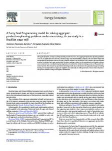
under-achievement of the ith goal. Despite MSGP model allows DMs to set multiple coefficients mapping each one decision variable in the left-hand-side of the constraints, however, there are nonetheless some drawbacks as follows. Let us consider a decision-making problem depicted in Fig. 1. Assume that there is a large rectangle S representing the global market and four small rectangles A, B, C and D representing the domain marketing corresponding to four different companies CA, CB, CC, CD, respectively. Each company sells two products and each product can be sold to two types of customers (e.g., general customer and member customer). Based on group pricing discrimination strategy (GPDS), each product has two different prices (one price is for general customer; the other is for member customer). Let us take the small rectangle (A) in Fig. 1 for instance to illustrate this idea. Suppose that g1 represents the sale goal of CA, and the DM of CA would like to find out the best quantities of products sold to the two types of customers under the goal g1.

Rectangle S {( p11 , p12 )x1} g1

{( p31 , p32 )x1} g2

{( p21 , p22 )x2} g1

{( p41 , p42 )x2} g2

Rectangle (A) Rectangle (B)

{( p51 , p52 )x1} g3

{( p71 , p72 )x1} g4

{( p61 , p62 )x2} g3

{( p81 , p82 )x2} g4

Rectangle (C) Rectangle (D)

Fig. 1. Example of MSGP coefficients To solve this problem, we can let the decision variable xi (i=1, 2) be the individual quantity on selling each of the two products, then define the coefficients pij(i, j=1, 2) are the two different prices for the two types of customer for ith product. That is, every decision variable (x1 and x2) in rectangle (A) has two associated coefficients. By referring to MSGP model, this problem can be expressed as follows. (1)  p11b1  p12 (1  b1 )x1   p21b2  p22 (1  b2 )x2  g1 where bi (i=1, 2) are binary variables, pij (i, j=1, 2) are two possible prices for two products, x1 and x2 are quantities sold of the two products. Rendering the result of Eq.(1) into Table 1 by corresponding to the behavior of two binary variables b1 and b2.

b2 1

0

Table 1.The result of MSGP b1 0

1

p12 x1  p 21 x 2  g1

p31 x1  p 41 x 2  g1

Fall in Rectangle (A)

Fall in Rectangle (B)

p52 x1  p 62 x 2  g1

p 71 x1  p82 x 2  g1

Fall in Rectangle (C)

Fall in Rectangle (D)

From Table 1, we realize that only one coefficient at a time can be chosen for each decision variable in the MSGP model. In other words, the relationship between all the possible coefficients for each decision variable is actually action as an exclusive-or (XOR) relationship [11]. This observation indicates that elements in the coefficients set of each constraint are mutual exclusive, and accordingly, are discrete and independent (actually not glued together). Hence, if the DM would like to solve a problem in which double coefficients might co-exist and co-affect each other at the same time, the solution of MSGP could not fully meet DM’s requirements. To the best knowledge of the author, no work has been done for solving such problem. Thus, the purpose of this study is to solve the problems of multiple coefficients existing in the GPDS and to establish a new articulated model that is still missing heretofore.

In sum, the above discussion reveals that we need to invent a new model to solve such problem where the relationship between the multiple coefficients mapping each decision variables can be an OR relationship not only a XOR relationship.

The OR relationship between the multiple coefficients for each decision variable should contain the XOR function plus the AND function. This significant improvement is the major contribution of the paper.

Table 2. The result of DCGP coefficients b1 b2

0

1

p12 t11  p11t12  p21t 21  p 22 t 22  g1

p31t 31  p32 t 32  p 41t 41  p 42 t 42  g1

Fall in Rectangle(A)

Fall in Rectangle (B)

p52 t 51  p51t 52  p62 t 61  p61t 62  g1

p71t 71  p72 t 72  p82 t 81  p81t 82  g1

Fall in Rectangle (C)

Fall in Rectangle (D)

1

0

III. MODELING MULTI-COEFFICIENTS GOAL PROGRAMMING PROBNLEM

GPDS is that a DM setting different prices for one single product in accordance with customer's property for maximizing profits or maximizing the quantities sold of products of an enterprise [25]. In fact, many enterprises often take this policy to enhance their competitiveness such as airline company, hotels, retailers, car rental agencies, travel, hospitality and entrainment industries [6][7][8][9][12][4][5][25]. In order to implement the OR relationship for multiple coefficients of GPDS, we try to derive a double-coefficients goal programming (DCGP) model as follows. The Fig.2 is revised from Fig.1, take the rectangle (A) in Fig. 2 for instance to demonstrate the OR relationship how to represent the multiple coefficients of GPDS. First, we introduce an additional decision variable tij, which indicates the quantity of product i sold to the specified customer group j. Other notations are defined as follows. pij: Selling price of ith product sold to jth type of customer (i=1, 2,…,8; j=1, 2) tij: Quantity Sold of ith product to jth type of customer (i=1, 2,…,8; j=1, 2) xi : total selling amount of ith product (i=1, 2,…,8) Rectangle S {[( p11 , p12 )t11; ( p11 , p12 )t12]x1} g1 {[( p31 , p32 )t31; ( p31 , p32 )t32]x3} g2 {[( p21 , p22 )t21; ( p11 , p12 )t22]x2} g1 {[( p41 , p42 )t41; ( p41 , p42 )t42]x4} g2 Rectangle (A)

binary variables b1 and b2 into the DCGP model to deal with this problem; the new model can be expressed as follows.

 p11b1  p12 (1  b1 ) t11   p11 (1  b1 )  p12b1 ) t12   p21b2  p22 (1  b2 ) t21   p21 (1  b2 )  p22b2  t22  g1 2

t j 1

ij

 xi (i  1, 2)

where bi (i=1, 2) are binary variables; x1 and x2 are quantities sold of the two products, respectively. Rendering the result of Eq.(2) into Table 2 by corresponding two binary variables b1 and b2. Figure 3 shows the difference between MSGP and DCGP model. As can be seen in Figure 3, each decision variable (xi) in the DCGP model can be decomposed into two ‘sub decision variables’ (ti1 and ti2), which represents two different types of customer, and each sub decision variable is mapping two different prices. In order to find out the proper price of each sub decision variable, we can add binary variables (bi) and its inverse (1-bi) to deal with this problem. Eq.(1) is then be transformed to Eq.(2). For example, if b1=1 and b2=1, then Eq.(2) becomes ” p11 t11  p12t12  p21t 21  p22t 22  g1 ”, or if b1=1 and b2=0, then Eq.(2) becomes ” p11 t11  p12 t12  p 22 t 21  p 21t 22  g1 ” . As can be seen, despite how the bi is changed, each tij can easily be mapped to a proper coefficient (pij) finally. That is, through this method, we can reach the “OR” relationship for the problem of DCGP.

Rectangle (B)

MSGP

{[( p51 , p52 )t51; ( p51 , p52 )t52]x5} g3 {[( p71 , p72 )t31; ( p71 , p72 )t72]x7} g4 {[( p61 , p62 )t21; ( p61 , p62 )t62]x6} g3 {[( p81 , p82 )t41; ( p81 , p82 )t82]x8} g4 Rectangle (C)

(2)

DCGP xi

xi ti1

Rectangle (D)

ti2

Fig. 2. Example of DCGP coefficients Second, we show how to find out the proper coefficient of each decision variable in the DCGP model. Following the idea of Chang (2007) and Liao (2009), we introduce two extra

pi1

pi2

pi1

pi2

pi1

pi2

Fig. 3. The difference between MSGP and DCGP model

n

From previous descriptions, we know that the relationship between all the possible coefficients of each decision variable can actually be an “OR” relationship, not only an “XOR” relationship. Subsequently, the general DCGP model can be expressed as follows.

min z   d i d i i 1

m

s.t

m

t

min z   d i d i

j 1

i 1

ij i

j 1 2

t j 1

ij

ij

( B) t ij  d i  d i  g i , i  1,2,...,n,

 xi i  1, 2, ..., n,

d i , d i  0, i  1, 2, ..., n,

s.t 2

ij ij

j 1

n

 p b

p c

 

cij ( B )  Ri ( x), i  1, 2, ..., n,



 pij (1  bi ) t ij  pij (1  bi )  pij bi t ij  d i  d i  g i , i  1, 2,, n

X  F ( F is a feasible set),

where cij(B) is a function of binary serial number by refereeing to chang (2007); Ri (x) is the function of resources limitations; other variables are defined as in DCGP.

 xi , i  1, 2,, n

d i , d i  0, i  1, 2, 3, n X  F ( F is a feasible set)

where bi is the binary variable; xi represents total selling amount 



of ith product; d i and d i

are, respectively, over- and

under-achievements of the ith goal. In general, if there are more than two prices mapping one product, it becomes a multi-coefficients GP (MCGP) problem. Furthermore, based on the conceptualization from the proposed DCGP model, we can add more extra binary variables for modeling MCGP. The MCGP model can be expressed as follows. Table 3. Selling price, purchasing cost and marketing cost of each product Product Name Item

TV General Customer

Member Customer

Radio General Member Customer Customer

Cell phone General Member Customer Customer

Selling Price

$10

$8

$7

$6

$6

$5

Purchasing Cost

$7

$7

$5

$5

$4

$4

Marketing Cost

$0.3

$0.4

$0.3

$0.4

$0.1

$0.2

IV. AN ILLUSTRATIVE EXAMPLE A wholesaler sells three products: TV, radio, and cellular phone. Each product can be sold to two types of customers, namely general customer and member customer. Therefore, the DM of the wholesaler company decided to deploy the GPDS for the three products. For each product, the selling price and related costs are described in Table 3. The DM wants to find out the best combination of quantities of the three products for general customer and member customer and satisfy the following pre-defined goals.  Goal 1 (Revenue Goal): The DM wishes that the revenue is greater than or equal to 250.  Goal 2 (Purchasing Cost Goal): The DM wishes that total purchase cost of acquiring three products is

smaller than or equal to 150.  Goal 3 (Marketing Cost Goal): The DM wishes that total marketing cost of the three products is smaller than or equal to 40. In addition to the above three major goals, the DM also wishes that among the total sales, 45 percentages is on TV selling, 30 percentages is on Radio selling, and 25 percentages is on Cellular Phone selling. In the meanwhile, the DM also hopes in extra that on selling each product, a 60 percentage ratio over all can be sold to the member customers. To illustrate the modeling and solving of the problem by DCGP, the related notations are defined as follows: x1: Total selling amount of TV x2: Total selling amount of Radio x3: Total selling amount of Cellular phone

t1j: Quantities Sold of TV to member customers or general customers (j=1, 2) t2j: Quantities Sold of Radio to member customers or general customers (j=1, 2) t3j: Quantities Sold of Cellular Phone to member customers or general customers (j=1, 2) p1j: Selling price of TV to member customers or general customers by referring to Table 3, the p11=10 and p12=8 p2j: Selling price of Radio to member customers or general customers by referring to Table 3, the p21=7 and p22=6 p3j: Selling price of Cellular phone to member customers or general customers by referring to Table 3, the p31=6 and p32=5 c1j: Marketing cost on selling TV to member customers or general customers by referring to Table 3, the c11=0.3 and c12=0.4 c2j: Marketing cost on selling Radio to member customers or general customers by referring to Table 3, the c11=0.2 and c12=0.3 c3j: Marketing cost on selling Cellular phone to member customers or general customers by referring to Table 3, the c31=0.1and c32=0.2 According to the above mentioned, the problem can be formulated as follows. Goals: (g1) {10, 8}x1 + {7, 6}x2 + {6, 5} x3 ≧ 250 (g2) 7x1 + 5x2 + 4x3 ≦ 150 (g3) {0.3, 0.4}x1 + {0.2, 0.3}x2 + {0.1, 0.2} x3 ≦ 40 Constraints: x1=0.45(x1 + x2 + x3), x2=0.3 (x1 + x2 + x3), x3=0.25 (x1 + x2 + x3), t11 + t12 =x1, t21 + t22 =x2, t31 + t32 =x3, where the { } braces is enclosing a set of some possible coefficients in an OR relationship (each stated { } set includes two coefficients that is to be appeared in XOR relationship or in AND relationship), as mentioned in Section 1. For example, for g1, there is a possible coefficient set {10, 8} beneath x1 as stated. In this case, rather than taking 10 or 8 individually,

either 10, 8, or a mixture of the both, are the possible coefficients of x1 and are supposed to affect the result. Based on the proposed DCGP model, this problem can be formulated as the following program: min z  d1  d 2  d 3 s.t (10b1  8(1  b1 )) t11  (8b1  10(1 b1 )) t12  (7b2  6(1  b2 )) t 21  (6b2  7(1  b2 )) t 22  (6b3  5(1  b3 )) t 31  (5b3  6(1  b3 )) t 32  d1  d1  250, 7 x1  5 x 2  4 x3  d 2  d 2  150, (0.4b1  0.3(1  b1 )) t11  (0.3b1  0.4(1 b1 )) t12  (0.3b2  0.2(1  b2 )) t 21  (0.2b2  0.3(1  b2 )) t 22  (0.2b3  0.1(1  b3 )) t 31  (0.1b3  0.2(1  b3 )) t 32  d1  d1  40 b1t11  (1  b1 )t12  (0.6b1 x1 )  (0.6(1  b1 ) x1 ) b2 t 21  (1  b2 )t 22  (0.6b2 x 2 )  (0.6(1  b2 ) x 2 ) b3 t 31  (1  b3 )t 32  (0.6b3 x3 )  (0.6(1  b3 ) x3 x1  0.45( x1  x 2  x3 ), x 2  0.3( x1  x 2  x3 ), x3  0.25( x1  x 2  x3 ), t11  t12  x1 , d i , d i  0,

t 21  t 22  x 2 ,

t 31  t 32  x3 ,

i  1, 2, 3

where b1, b2 and b3 are binary variables; x1, x2 and x3 are the total selling quantities of TV, Radio and Cellular Phone, respectively; {t11, t12}, {t21, t22}, {t31, t32} denote for actual quantities on selling general customers OR member customers 

for products TV(x1), Radio(x2) and Cellular Phone(x3); d i 

and d i are the positive and negative deviation variables, respectively. Solving the above DCGP modeled problem using LINGO on a PC 586 with 2GHz CPU [24], we obtain the optimal solutions as (x1, x2, x3, x11, x12, x21, x22, x31, x32, b1, b2, b3)=(15.56, 10.37, 8.64, 6.22, 9.34, 6.22, 4.15, 5.19, 3.45, 1, 0, 0) shown in Table 4, the goal deviations is shown in Table 5. As can be seen in Table 5, g1 is reaching the selling goal 250 (100%) exactly; g2 has reached a positive value (+45.37) over the purchase cost goal 150, while g3 has a value of 10.72 below the marketing cost goal 40. The total deviation value ( d1  d 2  d 3 ) of objective function z is 45.37.

Table 4. Solutions of Case I Product Name TV Item Quantities sold Total selling amount

Radio

Cell phone

Member customer

General customer

Member customer

General customer

Member customer

General customer

9.34

6.22

6.22

4.15

5.19

3.45

15.56

10.37

8.64

Table 5. The goal deviations of DCGP Goal g1

g2

d 1

d 1

d 2

d 2

d 3

d 3

Deviation value

0

0

45.37

0

0

29.28

Total deviation

0

0

45.37

0

29.28

0

Deviation variable

[3]

From above results, we can realize that based on the DCGP model, we not only obtains much better result on reaching or approaching the aspiration levels of the three goals, but also obtains the quantities of product sold to member customers and general customers.

[4]

[5] [6]

V. CONCLUSIONS

[7]

The traditional GP model allows each decision variable on the left-hand-side of each goal mapping only one coefficient. Practically, in some cases, one decision variable mapping multiple coefficients may exist in the real world such as GPDS problem. Although, past researches proposed a MSGP model, in which, each decision variable can map multiple coefficients. However, the relationship among these coefficients is an “XOR” relationship, not an “OR” relationship. Therefore, the MSGP model cannot solve a problem with multiple coefficients. In this study, we propose a new DCGP model to solve the “OR” relationship among multiple coefficients. In addition, we take a simple group pricing problem as an example to show the correctness and usefulness of the proposed model. In this example, the proposed model not only allows a DM can set different prices for one single product, but also, it obtains a proper satisfying solution in considering balance of all goal targets. Finally, the superiority of the proposed approach is observed from the proposed illustrative example We hope the promising result could advise us and motivate the need for further researches on the field of multiple choices goal programming henceforth.

[8]

REFERENCES

[22]

[1]

[2]

g3

Adeyeye, A D. (2008). Goal programming model for production planning in a toothpaste factory. South African journal of industrial engineering, 19(2), 197-209. Amiri, M. (2009). Developing and solving a new model for the location problems: Fuzzy-goal programming approach. Journal of applied sciences, 9(7), 1344-1349.

[9]

[10] [11] [12]

[13] [14] [15] [16]

[17] [18]

[19] [20] [21]

[23] [24] [25] [26]

Aouni, B., Kettani, O. (2001). Goal programming model: A glorious history and a promising future. European Journal of Operational Research, 133, 225-231. Bitran, G. R., & Mondschein, S. V. (1995). An application of yield management to the hotel industry considering multiple day stays. Operations Research, 43, 427–443. Bitran, G. R., & Gilbert, S. M. (1996). Managing hotel reservations with uncertain arrivals. Operations Research, 44, 35–49. Belobaba, P. P. (1987). Airline yield management: An overview of seat inventory control. Transportation Science, 21, 63–73. Belobaba, P. P. (1989). Application of a probabilistic decision model to airline seat inventory control. Operations Research, 37, 183–197 Belobaba, P. P., & Wilson, J. L. (1997). Impacts of yield management in competitive airline markets. Journal of Air Transport Management, 3, 3–9. Bernstein, F., & Federgruen, A. (2003). Pricing and replenishment strategies in a distribution system with competing retailers. Operations Research, 51, 409–426. Charnes A, Cooper WW. (1961). Management model and industrial application of linear programming. Vol. 1. Wiley, New York. Carl G. Hempel (1966), “Philosophy of Natural Science”, Prentice Hall. Chen, F., Federgruen, A., & Zheng, Y. S. (2001). Near-optimal pricing and replenishment strategies for a retail/distribution system. Operations Research, 49(6), 839–853. Chang, C. T. (2000). An efficient linearization approach for mixed integer problems. European Journal of Operational Research, 123, 652-659. Chang, C. T. (2007). Multi-choice goal programming. Omega: The International Journal of Management Science, 35(4), 389-396. Dolgui, A. (2010). Pricing strategies and models. Annual reviews in control, 34, 101-110. Giannikos, I. (2009). A fuzzy goal programming model for task allocation in teamwork. International Journal of Human Resources Development and Management, 9(1), 97-115. Ignizio JP. (1985). Introduction to linear goal programming. Beverly, Hills, CA: Sage. Ku, C.-Y. (2010). Global supplier selection using fuzzy analytic hierarchy process and fuzzy goal programming. Quality and quantity, 44(4), 623-640. Lee, S. M. (1972). Goal programming for decision analysis. Philadelphia, PA: Auerbach. Liao, C. N. (2009). Formulating the multi-segment goal programming. Computer & Industrial Engineering, 56, 138-141. Oddoye, J P. (2009). Combining simulation and goal programming for healthcare planning in a medical assessment unit. European journal of operational research, 193(1), 250-261. Pati, R K. (2008). A goal programming model for paper recycling system. Omega: 36(3), 405-417. Romero C. (2001). Extended lexicographic goal programming: a unifying approach. Omega;29:63-71. Scharge L. (2002). LINGO Release 8.0. LINDO System, Inc. Schön, C. (2010). On the optimal product line selection problem with price discrimination. Management science, 56(5), 896-902. Tamiz M, Jones D, Romero C. (1998). Goal Programming for decision making: an overview of the current state-of-the-art, European Journal of Operational Research;111:567-81.