Konuralp Journal of Mathematics c Volume 2 No. 1 pp. 45–62 (2014) °KJM
INTEGRAL TRANSFORM METHOD FOR SOLVING DIFFERENT F.S.I.ES AND P.F.D.ES A. AGHILI* AND M.R. MASOMI Abstract. In this work, the authors used Laplace transform to obtain formal solution to some systems of singular integral equations of fractional type. In the last section, the authors considered certain non homogeneous fractional system of heat equations with different orders which is a generalization to the problem of heat transferring from metallic bar through the surrounding media. Illustrative examples are also provided.
1. Introduction and Definitions Fractional differential equations have been the focus of many studies due to their frequent appearance in various fields such as chemistry and engineering, physics. The main reason for success of applications fractional calculus is that these new fractional order models are more accurate than integer order models, i.e. there are more degrees of freedom in the fractional order models. The Laplace transform technique is one of most useful tools of applied mathematics. Typical applications include heat transfer, diffusion, waves, vibrations and fluid motion problems. However, contrary to expectations, it is surprising to find that the popularity of Laplace transforms, in comparison to numerical or other methods, is gradually diminishing and Laplace transform is less fashionable today than they were a few decades ago. Nevertheless, the applications of Laplace transforms continue to be an important part of the mathematical education received by students in various fields of natural sciences and engineering. The fractional diffusion equation, the fractional wave equation, the fractional advection-dispersion equation, the fractional kinetic equation and other fractional PDEs have been studied and explicit solutions have been achieved by Mainardi, Pagnini and Saxena [18], Langlands [13], Mainardi, Pagnini and Gorenflo [17], Mainardi and Pagnini [15,16], Yu and Zhang [25], Liu, Anh, Turner and Zhang [14], Saichev and Zaslavsky [21], Saxena, Mathai and Haubold [22], Wyss [24] and several other research works can be found in other literatures. In these works, the techniques of using integral transforms were used to obtain the 1991 Mathematics Subject Classification. 26A33; 34A08; 34K37; 35R11. Key words and phrases. Caputo fractional derivative; Time fractional heat equation; Laplace transform; Fractional order singular integral equation system; Kelvin’s functions. The author is supported by university of Guilan. 45
46
A. AGHILI* AND M.R. MASOMI
formal solutions of fractional PDEs. Integral transforms are extensively used in solving boundary value problems and integral equations. The problem related to partial differential equations can be solved by using a special integral transform thus many authors solved the boundary value problems by using single Laplace transform. Laplace transform is very useful in applied mathematics, for instance for solving some differential equations and partial differential equations, and in automatic control, where it defines a transfer function. The Caputo fractional derivatives of order α > 0 (n − 1 < α ≤ n, n ∈ N ) is defined by Z t 1 f (n) (x) dx. Γ(n − α) a (t − x)α−n+1 The Laplace transform of a function f (t) denoted by F (s), is defined by the integral equation Z ∞ e−st f (t)dt := F (s). L{f (t)} = C α a Dt f (t)
=
0
Definition 1.1. The inverse Laplace transform is given by the contour integral Z c+i∞ 1 est F (s)ds, 2πi c−i∞ where F (s) is analytic in the region Re(s) > c. f (t) =
Theorem 1.1. For n − 1 < α ≤ n, we can get α L{C 0 Dt f (t)}
α
= s F (s) −
n−1 X
sα−k−1 f (k) (0).
k=0
Two-parameter Mittag-Leffler function and Wright function is given by Eα,β (z) = W (α, β; z) =
∞ X
zn , Γ(αn + β) n=0 ∞ X
zn . n!Γ(αn + β) n=0
when α, β, z ∈ C. Theorem 1.2. Schouten-Van der Pol Theorem: Consider a function f (t) which has the Laplace transform F (s) which is analytic in the half-plane Re(s) > s0 . We can use this knowledge to find g(t) whose Laplace transform G(s) equals F (φ(s)), where φ(s) is also analytic for Re(s) > s0 . This means that if Z ∞ G(s) = F (φ(s)) = f (τ ) exp(−φ(s)τ )dτ, 0
and 1 g(t) = 2πi then
Z
c+i∞
F (φ(s)) exp(ts)ds, c−i∞
INTEGRAL TRANSFORM METHOD FOR SOLVING DIFFERENT F.S.I.ES AND P.F.D.ES 47
Z g(t) =
µ
∞
f (τ ) 0
1 2πi
Z
c+i∞
¶ exp(−φ(s)τ ) exp(ts)ds dτ.
c−i∞
Proof. See [10] 2. Fractional Order Singular Integral Equations The mathematical formulation of physical phenomena often involves Cauchy type, or more severe, singular integral equations. There are many applications in many important fields, like fracture mechanics, elastic contact problems, the theory of porous filtering contain integral and integro- differential equation with singular kernel. In following section, Laplace transform has been used to solve certain types of singular integral equations of fractional order. We solve a fractional order singular integral equation system. Special examples are mentioned. Lemma 2.1. The fractional Fredholm singular integro-differential equation of the form Z (2.1)
C α 0 Dx ϕ(x)
= f (x) + λ 0
∞
√ x ν ( ) 2 Jν (2 xt)ϕ(t)dt, t
where ϕ(0) = 0, 0 ≤ α ≤ 1 and ν > −1 has the formal solution as (2.2)
ϕ(x) =
1 2πi
Z
c+i∞
c−i∞
λ F ( 1s ) sx s−α F (s) + sν+1 e ds. 2 1−λ
Proof. Let L(ϕ(x)) = Φ(s) and L(f (x)) = F (s), then by using the Laplace transform of (2-1) we have the following relation 1 1 Φ( ). sν+1 s In relation (2-3) we replace s by 1s , to obtain
(2.3)
sα Φ(s) = F (s) + λ
1 1 s−α Φ( ) = F ( ) + λsν+1 Φ(s). s s Combination of (2-3) and (2-4), Φ(s) can be obtained as
(2.4)
λ s−α F (s) + sν+1 F ( 1s ) . 1 − λ2 By using the complex inversion formula, relation (2-5) leads to the following,
(2.5)
Φ(s) =
1 ϕ(x) = 2πi
Z
c+i∞
c−i∞
λ F ( 1s ) sx s−α F (s) + sν+1 e ds. 1 − λ2
Example 2.1. Solve the following fractional singular integral equation Z ∞ √ 2 x 1 1 C 3 +λ ( ) 4 J 12 (2 xt)ϕ(t)dt, 0 Dx ϕ(x) = √ t πx 0 Solution. By using the formula (2-2), we get
48
A. AGHILI* AND M.R. MASOMI
ϕ(x)
= =
1 2πi
Z
c+i∞
2
s− 3 F (s) + 1−
c−i∞
λ
3
s2 λ2
F ( 1s )
esx ds =
1 2πi
Z
c+i∞
c−i∞
1
7
s6
+
λ s
1 − λ2
esx ds
1 6
1 x ( + λ). 1 − λ2 Γ( 67 )
Lemma 2.2. The system of fractional Fredholm singular integro-differential equation of the form Z ∞ √ x ν C α D ϕ (x) = f (x) + λ ( ) 2 Jν (2 xt)ϕ2 (t)dt, 0 x 1 t 0 Z ∞ √ x µ C α ( ) 2 Jµ (2 xt)ϕ2 (t)dt, 0 Dx ϕ2 (x) = g(x) + λ t 0 where ϕ1 (0) = ϕ2 (0) = 0 and 0 < α, β ≤ 1 has the formal solutions (2.6) ϕ1 (x) =
1 2πi
Z
c+i∞
µ
µ s−α F (s) +
c−i∞
1 ϕ2 (x) = 2πi
(2.7)
Z
c+i∞ c−i∞
λ2 G(s) 1 − λ2 sν−µ
¶ +
¶ λ 1 1 G( ) exs ds, 1 − λ2 sν+1 s
λ s−α G(s) + sµ+1 G( 1s ) xs e ds. 1 − λ2
Proof. Applying the Laplace transform term wise to both equations and using the initial conditions yields sα Φ1 (s) = F (s) +
(2.8)
λ 1 Φ2 ( ), sν+1 s
λ 1 Φ2 ( ). sµ+1 s Following the same procedure as in lemma 2.1, we get Φ2 (s) as sα Φ2 (s) = G(s) +
(2.9)
Φ2 (s) = then, changing s to
1 s
λ s−α G(s) + sµ+1 G( 1s ) , 2 1−λ
leads to
sα G( 1s ) + λsµ+1 G(s) 1 Φ2 ( ) = . s 1 − λ2 1 By replacing Φ2 ( s ) in (2-8), we will have µ ¶ λ2 G(s) λ 1 1 Φ1 (s) = s−α F (s) + + G( ). 1 − λ2 sν−µ 1 − λ2 sν+1 s At this point, using the complex inversion formula, the final solutions are as follows 1 ϕ1 (x) = 2πi
Z
c+i∞
µ s
c−i∞
−α
µ F (s) +
λ2 G(s) 1 − λ2 sν−µ
¶ λ 1 1 + G( ) ex s ds, 1 − λ2 sν+1 s
INTEGRAL TRANSFORM METHOD FOR SOLVING DIFFERENT F.S.I.ES AND P.F.D.ES 49
1 ϕ2 (x) = 2πi
Z
c+i∞ c−i∞
λ s−α G(s) + sµ+1 G( 1s ) xs e ds. 1 − λ2
Example 2.2. Let us solve the system Z ∞ 1 √ e− 4x x 3 = √ +λ ( ) 4 J 32 (2 xt)ϕ2 (t)dt, 3 t 2 πx 0 Z ∞ √ 1 x 1 C 2 ( ) 4 J 21 (2 xt)ϕ2 (t)dt, 0 Dx ϕ2 (x) = 1 + λ t 0 where ϕ1 (0) = ϕ2 (0) = 0 and 0 < α, β ≤ 1. Direct use of relations (2-6) and (2-7), leads to 1
C 2 0 Dx ϕ1 (x)
( ϕ1 (x)
= L
−1
√ s
e− √
λ2 1 λ 1 + + 1 − λ2 s 25 1 − λ2 s 32 s
1
3
)
1
e− 4x 4λ2 x 2 2λx 2 √ + √ +√ , πx 3 π(1 − λ2 ) π(1 − λ2 )
=
( ϕ2 (x) = L
−1
3
1
s− 2 + λs− 2 1 − λ2
) =
1 √2 x 2 π
√λ πx λ2
+
1−
.
2.1. Evaluation of the Integrals. In applied mathematics, the Kelvin functions Berν ( x ) and Beiν ( x ) are the real and imaginary parts, respectively, of Jν (xe3πi/4 ),where x is real, and Jν (z) is the ν-th order Bessel function of the first kind. Similarly, the functions Kerν ( x ) and Keiν ( x ) are the real and imaginary parts, respectively, of Kν (xeπi/4 ), where Kν (z)is the ν-th order modified Bessel function of the second kind. These functions are named after William Thomson, 1st Baron Kelvin. The Kelvin functions were investigated because they are involved in solutions of various engineering problems occurring in the theory of electrical currents, elasticity and in fluid mechanics. One of the main applications of Laplace transform is evaluating the integrals as discussed in the following. Lemma 2.3. The following integral relationship holds true Z
∞ 1
√ π bei( 2λ)dλ √ = J0 (1)I0 (1). 2 2 λ −1
Proof. Let us define the following function Z
∞
I(x) = 1
√ bei( 2xλ)dλ √ . λ2 − 1
Laplace transform of I(x) leads to Z
ÃZ
∞
L{I(x)} =
e 0
∞
−sx 1
! √ bei( 2xλ)dλ √ dx. λ2 − 1
By changing the order of integration, which is permissible, we obtain
50
A. AGHILI* AND M.R. MASOMI
Z
∞
√
L{I(x)} = 1
or
µZ
1
e
λ2 − 1 Z
∞
−sx
¶ √ bei( 2xλ)dx dλ,
0
∞
1 λ ( sin )dλ. 2s −1 s 1 At this point, let us introduce the new variable λ = cosh ξ, we get the following Z 1 ∞ sin((2s)−1 cosh ξ)dξ, L{I(x)} = s 0 using the following well-known integral representation for J0 (ϕ) Z 2 ∞ J0 (ϕ) = sin(ϕ cosh ϑ)dϑ. π 0 One gets finally √
L{I(x)} =
1
λ2
π 1 J0 ( ), 2s 2s now, taking inverse Laplace transform of the above relationship leads to L{I(x)} =
I(x) = L−1 { Letting x = 1 we get Z
∞ 1
√ √ π 1 π J0 ( )} = J0 ( x)I0 ( x). 2s 2s 2
√ bei( 2λ)dλ π √ = J0 (1)I0 (1). 2 2 λ −1
Lemma 2.4. The following integral relations hold true Z
√ 1 1 xµ−1 ber(2 ln x)dx = cos , µ µ √ Z 1 ber(2 ln x) √ dx = 2 cos 2. x 0
1
0
Proof. Let us define the following function Z
1
I(ξ) =
xµ−1 ber(2
p (ln x)ξ)dx.
0
Laplace transform of I(ξ) leads to µZ Z ∞ L{I(ξ)} = e−sξ
1
xµ−1 ber(2
¶ p (ln x)ξ)dx dξ.
0
0
By changing the order of integration, which is permissible, we will have Z
1
L{I(ξ)} = 0
Z xµ−1
∞
e−sξ ber(2
p
(ln x)ξ)dξdx.
0
But the value of inner integral is as following Z ∞ p (ln x) 1 e−sξ ber(2 (ln x)ξ)dξ = cos . s s 0
INTEGRAL TRANSFORM METHOD FOR SOLVING DIFFERENT F.S.I.ES AND P.F.D.ES 51
To prove the second relationship, by setting this value in the integral, one gets Z
1
L{I(ξ)} = 0
1 (ln x) 1 xµ−1 cos dx = s s s
Z
1
xµ−1 cos
0
(ln x) dx. s
At this point, we introduce the new variable ln x = −w. One gets after easy calculation L{I(ξ)} =
Z
1 s
∞ 0
1 s w e−µw cos( )dw = { 2 }. s µ s + (µ−1 )2
Taking inverse Laplace transform to obtain Z I(ξ) =
1
xµ−1 ber(2
0
p ξ 1 (ln x)ξ)dx = cos , µ µ
from the above relationship, we get Z
√ 1 1 xµ−1 ber(2 ln x)dx = cos . µ µ
1
I(1) = I0 (µ) = 0
In the above integral, by setting 0.5 for the parameter,we obtain the second assertion Z
√ ber(2 ln x)dx √ = 2 cos 2. x
1
I0 (0.5) = 0
3. Bobylev-Cercignani Theorem and Their Applications Bobylev and Cercignani developed a theorem [8] concerning the inversion of multivalued transforms that are analytic everywhere in the s− plane except along the negative real axis. The theorem is as follows: Theorem 3.1. Bobylev-Cercignani Theorem: Let f (t) denote a real-valued function, where its Laplace transform F (s) exists. Let F (s) satisfy the following hypothesis: 1) F (s) is a multi-valued function which has no singularities in the cut s− plane. The branch cut lies along the negative real axis (−∞, 0]. 2) F ∗ (s) = F (s∗ ), where the star denotes the complex conjugate. 3) F ± (η) = lim F (ηe±φi ) and F + (η) = (F− (η))∗ . φ→π −
1 4) F (s ) = o(1) as |s| → ∞ and F (s) = o( |s| ) as |s| → 0, uniformly in any sector | arg(s)| < π − η, 0 < η < π. ±φi ) ∈ L1 (R+ ) 5) There exists ε > 0, such that for every π − ε < φ ≤ π, F (re 1+r ±φi −δr and |F (re )| < a(r), where a(r) does not depend on φ and a(r)e ∈ L1 (R+ ) for any δ > 0.Then
1 f (t) = π
Z
∞
Im( F − (η))e−tη dη.
0
In following lemma, we apply this theorem.
52
A. AGHILI* AND M.R. MASOMI
Lemma 3.1. The following relationship holds true ( L
−1
à r !) Z 1 µ + sα 1 ∞ exp −x = Im(F − (η))e−tη dη. s+1 λ + sα π 0
where 0 < α < 1, λ, µ > 0 and −
Im(F (η)) =
e
−x
q
ρ1 ρ2
cos(
θ1 −θ2 2
)
η−1
µ r ¶ θ1 − θ2 ρ1 sin x sin( ) . ρ2 2
Proof. F (s) satisfies all of the conditions listed in the theorem 3.1. Then
−
F (η) = = =
−φi
lim F (ηe
Ã
1
η α e−παi + µ η α e−παi + λ
!
exp −x ηe−πi + 1 µ r ¶ 1 ρ1 i(θ1 −θ2 ) 2 exp −x e 1−η ρ2 µ r ¶ 1 ρ1 θ1 − θ2 θ1 − θ2 exp −x (cos( ) + i sin( )) , 1−η ρ2 2 2
φ→π
)=
s
where ρ1 =
p p η 2α + 2µη α cos πα + µ2 , ρ2 = η 2α + 2λη α cos πα + λ2 , µ
θ1 = − tan
−1
η α sin απ η α cos απ + µ
µ , θ2 = − tan
−1
η α sin απ η α cos απ + λ
¶ (0 < θ < π).
Image part of F − (η) is founded as −
Im(F (η)) =
e
−x
q
ρ1 ρ2
cos(
θ1 −θ2 2
η−1
)
µ r ¶ ρ1 θ1 − θ2 sin x sin( ) . ρ2 2
Finally, the inverse Laplace transform is as f (t) =
1 π
Z
∞
Im(F − (η))e−tη dη.
0
Problem 1. Let us consider the following four terms partial fractional differential equation ∂ ∂ α u(x, t) ∂ β u(x, t) ∂u(x, t) { } + a = λu(x, t) − b , α β ∂x ∂t ∂t ∂x where 0 < α < 1, 0 < β ≤ 1, 0 < x < ∞, t, a, b > 0 with the boundary conditions u(0, t) =
tγ−1 (γ > 0), lim |u(x, t)| < ∞, x→∞ Γ(γ)
and the initial conditions u(x, 0) = ux (x, 0) = 0.
INTEGRAL TRANSFORM METHOD FOR SOLVING DIFFERENT F.S.I.ES AND P.F.D.ES 53
Solution. Applying the Laplace transform of the equation and using the boundary and initial conditions leads to differential equation with respect to x as asβ − λ U (x, t) = 0, sα + b when L{u(x, t)} = U (x, s). Solution of the above equation yields µ ¶ asβ − λ 1 . U (x, s) = γ exp −x α s s +b U (x, s) satisfies all of the conditions explained in the theorem 3.1. Hence Ux (x, t) +
µ ¶ aη β e−πβi − λ 1 U (x, η) = lim U (x, ηe ) = γ −πγi exp −x α −παi φ→π η e η e +b µ ¶ eπγi (aη β e−πβi − λ)(η α eπαi + b) = exp −x , ηγ ρ −
−φi
where ρ = η 2α + 2bη α cos πα + b2 . Therefore Im(U − (x, η)) = ½ ¾ 1 abη β cos βπ + aη α+β cos(α − β)π − λη α cos απ − λb exp −x ηγ ρ ½ ¾ α+β aη sin(α − β)π − abη β sin βπ − λη α sin απ × sin πγ − x . ρ Finally, u(x, t) is found to be Z 1 ∞ u(x, t) = Im( U − (x, η))e−tη dη. π 0 4. Partial Fractional Differential Equation (PFDE) with Moving Boundary In PFDE problems, Laplace transforms are particularly useful when the boundary conditions are time dependent. We consider now the case when one of the boundaries is moving. This type of problem arises in combustion problems where the boundary moves due to the burning of the fuel [10]. Such fractional partial differential equations have not been studied in the literature. Problem 2. Let us solve the following three terms time-fractional heat equation with moving boundaries 2 ∂u(x, t) ∂ α u(x, t) 2 ∂ u(x, t) = a +λ (0 < α ≤ 1), α 2 ∂t ∂x ∂x where λ ∈ R, βt < x < ∞, t > 0 and subject to the boundary conditions ¯ ¯ 1 1 u(x, t) ¯¯ = √ exp(− ), lim |u(x, t)| < ∞, x = βt 4t x→∞ πt and the initial condition u(x, 0) = 0 (0 < x < ∞).
(4.1)
54
A. AGHILI* AND M.R. MASOMI
Solution: We introduce the change of variable η = x − βt. The above equation can be reformulated as ¢ ∂ 2 w(η, t) ∂ α w(η, t) ∂ ¡ 1−α ∂w(η, t) w(η, t) = a2 −β +λ , 0 It α ∂t ∂η ∂η 2 ∂η
(4.2)
where 0 < η < ∞, t > 0 subject to the boundary conditions 1 1 w(0, t) = √ exp(− ), lim |w(η, t)| < ∞, 4t η→∞ πt and the initial condition w(η, 0) = 0 (0 < η < ∞). By applying the Laplace transform of the equation (4-2), we obtain ∂ 2 W (η, s) 1 β ∂W (η, s) sα + ( + λ) − 2 W (η, s) = 0, ∂η 2 a2 s1−α ∂η a
(4.3)
with conditions √ s
e− W (0, s) = √
, lim |W (η, t)| < ∞. s η→∞ Differential equation (4-3) has the solution as Ã
√ s
e− W (η, s) = √
λη βη η exp − 2 − 2 1−α − 2a 2a s 2 s
r
1 β 4sα ( 1−α + λ)2 + 2 4 a s a
! .
Case 1: If α = 1, then W (η, s) = e
η −(λ+β) 2a 2
Ã
√ s
e− √
η exp − a s
r
! 1 (β + λ)2 + s . 4 a2
Using the fact that ( L
−1
Ã
η exp − a
r
!) η2 2 1 η 1 2 (β + λ) + s = e− 4a2 (β+λ) t √ e− 4 a 2 t , 2 3 4a 2a πt
and using the Laplace transform inversion and then applying the convolution theorem in this transform, we get w(η, t) as w(η, t)
= L−1 {W (η, s)}
=
Z
η −(λ+β) η2 2a e 2aπ
0
t
1
e− 4(t−τ ) − 12 β+λ)2 τ − η22 p e 4a e 4 a τ dτ. τ 3 (t − τ )
Therefore we obtain u(x, t) as following x − βt −(λ+β) x−βt 2a2 u(x, t) = e 2aπ Case 2: If α 6= 1, then
Z 0
t
1
2 e− 4(t−τ ) − 12 (β+λ)2 τ − (x−βt) p e 4a e 4a2 τ dτ. τ 3 (t − τ )
INTEGRAL TRANSFORM METHOD FOR SOLVING DIFFERENT F.S.I.ES AND P.F.D.ES 55
W (η, s) = e
λη − 2a 2
à ! r √ 1 βη η β2 2βλ 4sα √ exp − s − 2 1−α − + 4 1−α + 2 + λ2 , 2a s 2 a4 s2−2α a s a s
and we can use the theorem 3.1, hence λη
−
W (η, ξ) = lim W (η, ξe
−φi
φ→π
− πi 2
×
s
Ã
βη η exp − 2 1−α (α−1)πi − 2 2a ξ e λη
π
e− 2a2 ei( 2 − √ = ξ
Ã
√ ξ)
exp
β2 2βλ 4ξ α e−απi + 4 1−α (α−1)πi + + λ2 4 2−2α (2α−2)πi a2 a ξ e a ξ e
η βηe−απi − 2 1−α 2a ξ 2
s β 2 e−2απi 4ξ α 2βλ + ( − 4 1−α )e−απi + λ2 4 2−2α 2 a ξ a a ξ
λη
π
√
e− 2a2 ei( 2 − √ = ξ
e
√
e− 2a2 e ξe )= √ − πi ξe 2
βη(cos απ−i sin απ) − η2 2a2 ξ1−α
rh
α β 2 cos 2απ +( 4ξ a2 a4 ξ2−2α
λη
π
e− 2a2 ei( 2 − √ = ξ
−
2βλ a4 ξ1−α
√ ξ)
e
!
!
ξ)
×
i h 2 2απ 4ξα ) cos απ+λ2 −i β 4 sin 2−2α +( a2 − a ξ
√ θi βη(cos απ−i sin απ) − η2 ρe 2 2a2 ξ1−α
2βλ a4 ξ1−α
i ) sin απ
,
where s½ ρ=
4ξ α 2βλ β 2 cos 2απ + ( 2 − 4 1−α ) cos απ + λ2 4 2−2α a ξ a a ξ
θ = − tan−1
β 2 sin 2απ a4 ξ 2−2α β 2 cos 2απ a4 ξ 2−2α +
α
+ ( 4aξ2 − α
( 4ξ a2 −
¾2
½ +
β 2 sin 2απ 4ξ α 2βλ + ( 2 − 4 1−α ) sin απ 4 2−2α a ξ a a ξ
2βλ a4 ξ 1−α ) sin απ 2βλ 2 ) cos απ + λ 4 1−α a ξ
(0 < θ < π).
Then imaginary part of W − (η, ξ) is λη
p e− 2a2 βη cos απ − η √ρ cos θ2 βη η√ θ Im(W (η, ξ)) = √ e 2a2 ξ1−α 2 cos( ξ + 2 1−α sin απ + ρ sin ). 2a ξ 2 2 ξ −
The formal solution will be as follows, 1 u(x, t) = π
Z
∞ 0
Im(W − (x − βξ, ξ))e−tξ dξ.
¾2
56
A. AGHILI* AND M.R. MASOMI
5. A Non-Homogenous System of Fractional Heat equations with different orders In this section, we consider certain non-homogeneous fractional system of heat equations (different orders) which is a generalization to the problem of heat transferring from metallic bar through the surrounding media studied by V.A. Ditkin, P.A. Prudnikov [9]. The basic goal of this work has been to implement the Laplace transform method for studying the above mentioned problem. The goal has been achieved by formally deriving exact analytical solution. Problem 3. We consider the following system of fractional PDE with different orders in Caputo sense (5.1)
c
Dtα u
¯ ∂2u ∂v ¯¯ + γu = 1 + , + λa ∂x2 ∂r ¯ r = a
∂ 2 v 1 ∂v + , ∂r2 r ∂r where 0 < α, δ < 1, t > 0, −l ≤ x ≤ l, r ≥ a and β, γ ∈ R with the boundary conditions (5.2)
c
Dtδ v − βv =
u(x, 0) = v(x, r, 0) = 0, u(−l, t) = u(l, t) = 0, and v(x, a, t) = u(x, t), lim v(x, r, t) = 0. r→∞
Solution: By taking the Laplace transform of relation (5-2), we get p r2 Vrr + rVr + (i sδ − β)2 r2 V = 0. Let us assume that L{v(x, r, t)} = V (x, r, s), then one has p p V (x, r, s) = c1 J0 (i sδ − βr) + c2 Y0 (i sδ − βr), where J0 and Y0 are Bessel functions of the first and second kind of order zero, respectively. Using this fact that lim v(x, r, t) = 0, we get r→∞ p V (x, r, s) = c1 J0 (i sδ − βr). But v(x, a, t) = u(x, t), therefore p J0 (i sδ − βr) p U (x, s), V (x, r, s) = J0 (i sδ − βa) where L{u(x, t)} = U (x, s). On the other hand, we have ! à p ¯ p ∂V ¯¯ J1 (i sδ − βa) δ p . = U (x, s) −i s − β ∂r ¯ r = a J0 (i sδ − βa) Applying the Laplace transform term wise to relation (5-1), we obtain p p J1 (i sδ − βa) 1 α δ p s U = Uxx − iλa s − β U + − γU, s J0 (i sδ − βa)
INTEGRAL TRANSFORM METHOD FOR SOLVING DIFFERENT F.S.I.ES AND P.F.D.ES 57
or 1 Uxx − h(s)U = − , s
(5.3) where
p J (i sδ − βa) 1 p . h(s) = s + γ + iλa sδ − β J0 (i sδ − βa) Differential equation (5-3) has the following solution p
α
p
p h(s)x) + c2 sinh( h(s)x) +
1 . sh(s) Using the boundary conditions u(−l, t) = u(l, t) = 0 leads to à ! p cosh( h(s)x) 1 p U (x, s) = 1− . sh(s) cosh( h(s)l) U (x, s) = c1 cosh(
Let us assume that p cosh( h(s)x) p F (x, h(s)) = 1 − , cosh( h(s)l) then we get U (x, s) =
F (x, h(s)) . sh(s)
Now, if Lt {φ(x, t)} =
F (x, s) e−ξh(s) , Lt {ψ(ξ, t)} = , s s
then u(x, t) =
L−1 t {U (x, s)}
=L
−1
F (x, h(s)) { }= sh(s)
Z
∞
ψ(ξ, t)φ(x, ξ)dξ. 0
Finally, we will have φ(x, t) =
L−1 t {
F (x, s) } = L−1 t s ½
=
1−
=
1−
L−1 t ∞ X n=0
= Also,
½
√ cosh( sx) √ s cosh( sl) ½
L−1 t
¾ √ 1 cosh( sx) √ ) (1 − s cosh( sl) ( ¾ =1−
L−1 t
e
√ s(x−l)
√
1 + e−2 sx √ s(1 + e−2 sl )
)
√ ¾ √ exp(−((2n + 1)l − x) s) exp(−((2n + 1)l + x) s) − s s
¶ ∞ µ X (2n + 1)l − x (2n + 1)l + x √ √ 1− erf c( ) − erf c( ) . 2 t 2 t n=0
58
A. AGHILI* AND M.R. MASOMI
Figure 1
α
h(s) = s + γ + iλa
p
sδ
p J1 (i sδ − βa) p −β , J0 (i sδ − βa)
hence e−ξh(s) } s ( !) à p −ξsα δ − βa) p e J (i s 1 p = L−1 e−ξγ exp −iξλa sδ − β t s J0 (i sδ − βa) (p à !) p α δ − βa) p sδ − β e−ξs J (i s 1 −ξγ −1 p p = e Lt exp −iξλa sδ − β . s sδ − β J0 (i sδ − βa)
ψ(ξ, t) = L−1 t {
Case 1: Assume that δ = 1, therefore √ µ ¶¾ p J1 (i s − βa) 1 √ √ f1 (ξ, t) = exp −iξλa s − β s−β J0 (i s − βa) ½ µ √ ¶¾ √ J1 (i sa) 1 √ √ = eβt L−1 exp −iξλa s . t s J0 (i sa) ½
L−1 t
The inverse Laplace transform is given by ½ L−1 t
µ µ √ ¶¾ √ ¶ Z c+i∞ √ J (i sa) √ J1 (i sa) ts 1 1 1 √ exp −iξλa s 1 √ √ √ = exp −iξλa s e ds. 2πi c−i∞ s J0 (i sa) s J0 (i sa)
The integrand has a branch point at the origin and it is thus necessary to choose a contour which does not contain the origin. We deform the Bromwich contour so that the circular arc BDE is terminated just short of the horizontal axis and the arc LN A starts just below the horizontal axis. In between the contour follows an inclined path EH followed by a circular arcHJK enclosing the origin and a return section KL meeting the arc LN A (see figure). As there are no singularities inside this contour C, we have µ √ ¶ Z √ J (i sa) ts 1 √ exp −iξλa s 1 √ e ds = 0. s J0 (i sa) C
INTEGRAL TRANSFORM METHOD FOR SOLVING DIFFERENT F.S.I.ES AND P.F.D.ES 59
Now on BDE and LN A, we get ¯ µ ¶¯ √ ¯ 1 ¯ √ ¯ √ exp −iξλa s J1 (i√sa) ¯ ≤ √1 , ¯ s J0 (i sa) ¯ s so that the integrals over these arcs tend to zero as R → ∞. Over the circular arc HJK as its radius ε → 0, we have s = εeiθ , φ ≤ θ ≤ −φ. Thus µ ¶ √ Z √ J (i sa) ts 1 √ exp −iξλa s 1 √ lim e ds = 0. J0 (i sa) R → ∞ HJK s ε→0 √ √ iφ Along EH, s = ueiφ , s = ue 2 , hence µ ¶ √ Z √ J (i sa) ts 1 √ exp −iξλa s 1 √ lim e ds = s J0 (i sa) EH R→∞ ε → 0, φ → π µ ¶ √ Z ∞ √ J1 ( ua) −tu 1 √ exp −ξλa u √ e du. i u J0 ( ua) 0 √ √ iφ Similarly, along KL, s = ue−iφ , s = ue− 2 , then µ ¶ √ Z √ J1 (i sa) ts 1 √ exp −iξλa s √ lim e ds = s J0 (i sa) KL R→∞ ε → 0, φ → π µ ¶ √ Z ∞ √ J ( ua) −tu 1 √ exp −ξλa u 1 √ e du. i u J0 ( ua) 0 Consequently, we have µ ¶ √ Z Z √ J (i sa) ts 1 1 1 √ exp −iξλa s 1 √ e ds = ds + ds 2πi AB 2πi BDE s J0 (i sa) C Z Z Z Z 1 1 1 1 + ds + ds + ds + ds = 0. 2πi EH 2πi HJK 2πi KL 2πi LN A The final result is as 1 2πi
Z
µ ¶ √ √ J (i sa) ts 1 √ exp −iξλa s 1 √ e ds = s J0 (i sa) c−i∞ µ ¶ √ Z √ J1 ( ua) −tu 1 ∞ 1 √ exp −ξλa u √ e du. π 0 u J0 ( ua)
1 2πi
Z
c+i∞
Thus we obtain √ µ ¶¾ p 1 J1 (i s − βa) √ exp −iξλa s − β s−β J0 (i s − βa) µ ¶ √ Z ∞ √ J1 ( ua) −tu 1 1 βt √ √ e exp −ξλa u e du. π u J0 ( ua) 0 ½
f1 (ξ, t) = =
L−1 t
√
In case of 0 < δ < 1, we get
60
A. AGHILI* AND M.R. MASOMI
( f2 (ξ, t)
=
L−1 t
=
1 t
Z
∞
Ã
!) p δ − βa) p J (i s 1 p p exp −iξλa sδ − β sδ − β J0 (i sδ − βa) 1
f1 (ξ, τ )W (−δ, 0; −τ t−δ )dτ.
0
Also, for 0 < δ < 1, (p f3 (t) =
=
L−1 t ∞ X
sδ − βe−ξs s µ
1 2
n
(−β)
=
∞ X
µ
1 2
n
(−β)
n
n=0
=
∞ X
µ
1 2
(−β)n
n δ o α 1 = L−1 s 2 −1 (1 − βs−δ ) 2 e−ξs t α
δ
−δn+ 2 −1 −ξs L−1 e } t {s
(
¶ L−1 t ¶(
n
n=0
)
n
n=0
α
s
−δn+ δ2 −1
∞ X (−ξ)k sαk k=0
∞ X (−ξ)k
k!
k=0
)
k! δ
tδn−αk− 2 Γ(δn − αk − 2δ + 1)
) .
Consequently 1 −ξγ ψ(ξ, t) = L−1 t { exp(−ξh(s))} = e s
Z
t
f2 (ξ, η)f3 (t − η)dη : 0 < α, δ < 1 0
Finally, we obtain u(x, t) as follows Z u(x, t) =
∞
ψ(ξ, t)φ(x, ξ)dξ µZ t ¶ Z ∞ e−ξγ f2 (ξ, η)f3 (t − η)dη 0
=
0
0
Ã
¶! ∞ µ X (2n + 1)l − x (2n + 1)l + x √ √ × 1− erf c( ) − erf c( ) dξ. 2 ξ 2 ξ n=0 Now, we should determine the inverse Laplace transform of the following term p J0 (i sδ − βr) p V (x, r, s) = U (x, s) . J0 (i sδ − βa) If δ = 1, we obtain √ ¾ ∞ J0 (i s − βr) 2 X λk J0 ( λak r) λ2 √ g1 (r, t) = = 2 exp(−( 2k − β)t), a J1 (λk ) a J0 (i s − βa) k=0 √ where λ1 , λ2 , λ3 , . . . are roots of J0 (i s − βa). For 0 < δ < 1, we conclude that ½
L−1 t
INTEGRAL TRANSFORM METHOD FOR SOLVING DIFFERENT F.S.I.ES AND P.F.D.ES 61
) p J0 (i sδ − βr) p J0 (i sδ − βa) Z ∞ 2 X λk J0 ( λak r) ∞ λ2 exp(−( 2k − β)τ )W (−δ, 0; −τ t−δ )dτ 2 a t J1 (λk ) a 0 k=0 ¯ ∞ ¯ ª 2 X λk J0 ( λak r) © ¯ −δ 2 L W (−δ, 0; −τ t ); τ → s ¯ ¯ s = λak2 − β a2 t J1 (λk ) k=0 Ã∞ ! ∞ 2 X λk J0 ( λak r) X (−a2 )n t−δn t J1 (λk ) Γ(−δn)(λ2k − a2 β)n+1 n=0 (
g2 (r, t) =
=
=
=
L−1 t
k=0 ∞
=
λk J0 ( λak r) 2X a2 t−δ E (− ). −δ,0 t J1 (λk )(λ2k − a2 β) λ2k − a2 β k=0
Therefore, Ã v(x, r, t) =
L−1 t {V Z
=
(x, r, s)} =
L−1 t
! p J0 (i sδ − βr) p U (x, s) J0 (i sδ − βa)
t
u(x, η)g2 (r, t − η)dη : 0 < α, δ < 1. 0
6. Acknowledgment The authors would like to thank the anonymous referee for helpful comments and suggestions. 7. Conclusion The paper is devoted to study and applications of Laplace transform. The main purpose of this work is to develop a method for finding formal solution of certain systems of Fredholm fractional singular integral equations of second kind, analytic solution of the time fractional heat equation and system of partial fractional differential equations with different orders, which is a generalization to certain types of problems in the literature. Numerous non trivial examples and exercises provided throughout the paper. We hope that it will also benefit many researchers in the disciplines of applied mathematics, mathematical physics and engineering. References [1] Aghili, A., Ansari, A. Solving partial fractional differential equations using the LAtransform. Asian-European journal of mathematics. Vol 3, No 2, 209-220, 2010. [2] Aghili, A., Masomi, M.R. Solution to time fractional partial differential equations and dynamical systems via integral transforms. Journal of Interdisciplinary Mathematics. Vol 14, Issue 5-6, 545-560, 2011. [3] Aghili, A., Masomi, M.R. Solution to time fractional partial differential equations via joint Laplace-Fourier transforms. Journal of Interdisciplinary Mathematics Volume 15, Issue 2-3, 121-135, 2012. [4] Aghili, A., Masomi, M.R. Integral transform method for solving time fractional systems
62
A. AGHILI* AND M.R. MASOMI
and fractional heat equation. Boletim da Sociedade Paranaense de Matemtica, Vol 32, No 1, pp 305-322, 2014. [5] Aghili, A., Masomi, M.R. Transform method for solving time-fractional order systems of nonlinear differential and difference equations. Antarctica J. Math., 10(3), 237-251, 2013. [6] Aghili, A., Masomi, M.R. The double Post-Widder inversion formula for two dimensional Laplace transform and Stieltjes transform with applications. Bulletin of Pure and Applied Sciences, Volume 30 E (Math and Stat.) Issue 2, 191-204, 2011. [7] Aghili, A., Salkhordeh Moghaddam, B. Laplace transform pairs of N-dimensions and second order linear partial differential equations with constant coefficients. Annales Mathematicae et Informaticae 35, 310, 2008. [8] Bobylev, A.V., Cercignani, C. The inverse Laplace transform of some analytic functions with an application to the eternal solutions of the Boltzmann equation. Appl. Math. Lett. 15, 807-813, 2002. [9] Ditkin, V.A., Prudnikov, A.P. Calcul operationnelle. Mir publisher. 1979. [10] Duffy, D.G. Transform methods for solving partial differential equations. Chapman and Hall/CRC, 2004. [11] Kartashov, E.M., Lyubov, B.Ya., Bartenev, G.M. A diffusion problem in a region with a moving boundary. Soviet Physics Journal, Vol 13, Issue 12, 1641-1647, 1970. [12] Kilbas, A.A., Srivastava, H.M., Trujillo, J.J. Theory and applications of fractional differential equations. Elsevier, 2006. [13] Langlands T. Solution of a modified fractional diffusion equation. Physica A, 367, 136-144, 2006. [14] Liu, F., Anh, V.V., Turner, I., Zhuang, P. Time fractional advection dispersion equation. Appl. Math. Computing, 13, 233-245, 2003. [15] Minardi, F., Pagnini, G. The role of the Fox-Wright functions in fractional sub-diffusion of distributed order. Comput. Appl. Math. Vol 207, Issue 2, 245-257, 2007. [16] Minardi, F., Pagnini, G. The Wright functions as solutions of the time fractional diffusion equations. Appl. Math. Comput. Vol 141, Issue 1, 51-62, 2003. [17] Minardi, F., Pagnini, G., Gorenflo, R. Some aspects of fractional diffusion equations of single and distributed order. J. Comput. Appl. Math. Vol 187, Issue 1, 295-305, 2007. [18] Mainardi, F., Pagnini, G., Saxena, R. K. Fox H-functions in fractional diffusion. J. Comput. Appl. Math. 178, 321-331, 2005. [19] Podlubny, I. Fractional differential equations. Academic Press, 1999. [20] Redozubov, D.B. The Solution of linear thermal problems with a uniformly moving boundary in a sSemiinfinite region. Sov. Phys. Tech. Phys., 5, 570574, 1960. [21] Saichev, A., Zaslavsky, G. Fractional kinetic equations: solutions and applications. Chaos. 7(4), 753-764, 1997. [22] Saxena, R.K., Mathai, A.M., Haubold, H.J. Solutions of certain fractional kinetic equations and a fractional diffusion equation. Math. Phys. 51, 103506, 2010. [23] Sneddon, I. Ulam, S. Stark, M. Operational Calculus in two variables and its applications. Pergamon Press Ltd, 1962. [24] Wyss, W. The fractional diffusion equation. Math. Phys. 27, 2782-2785, 1986. [25] Yu, R., Zhang, H. New function of Mittag-Leffler type and its application the fractional diffusion-wave equation. Chaos, Solitons Fract. Vol 30, Issue 4, 946-955, 2006.
Department of Applied Mathematics, Faculty of Mathematical Sciences, University of Guilan. P.O. Box, 1841, Rasht - Iran E-mail address:
[email protected] ,
[email protected]