Integrated Maximum Flow Algorithm for Optimal Response Time

2012 41st International Conference on Parallel Processing

Integrated Maximum Flow Algorithm for Optimal Response Time Retrieval of Replicated Data Nihat Altiparmak and Ali S¸aman Tosun Department of Computer Science University of Texas at San Antonio San Antonio, TX 78249 {naltipar,tosun}@cs.utsa.edu

to offering lower worst-case additive error, replication has many other advantages including better fault-tolerance and support for queries of arbitrary shape. Readers are directed to [43] for an in-depth comparison and analysis of replicated declustering schemes. Optimal response time retrieval problem of replicated data is first formulated in [18] along with a Ford-Fulkerson based maximum flow solution for homogeneous disk arrays located on a single site. [45] extended the problem by locating the homogeneous disk arrays on two different sites and proposed a black box maximum flow algorithm for this extended problem. Generalized optimal response time retrieval problem handling the heterogeneous disk arrays, initial loads of the disks, and more than two number of sites is formulated in [12]. Generalized problem is solved by performing multiple runs of a black box maximum flow algorithm [12]. Although the number of maximum flow calls are optimized using binary capacity scaling technique in [12], black box usage of maximum flow did not allow the conservation of previously calculated flows eliminating possible performance improvements. Deciding the retrieval schedule of a query is a time critical issue since the decision time is directly added to the response time of the query. In this paper, we propose two sequential, and one parallel integrated maximum flow algorithms to reduce this decision time for the generalized retrieval problem. We found out that integrated push-relabel based algorithms are superior to the integrated Ford-Fulkerson based algorithms for optimal response time retrieval problems. Our sequential integrated push-relabel algorithm runs up to 2.5X faster than the black box version proposed in [12], and the parallel integrated push-relabel implementation achieves up to 4.25X (∼3X on average) speed-up using two threads compared to the black box algorithm. The rest of the paper is organized as follows. In Section II, we present related background information and motivation behind this work. Section III describes the Ford-Fulkerson based integrated solution. Sequential push-relabel based integrated algorithm is provided in Section IV, and parallel integrated push-relabel implementation is explained in Section V. We evaluate the performance of the proposed algorithms in Section VI and conclude with Section VII.

Abstract—Efficient retrieval of replicated data from multiple disks is a challenging problem. Traditional retrieval techniques assume that replication is done at a single site using homogeneous disk arrays having no initial load or network delay. Recently, generalized retrieval algorithms are proposed to cover heterogeneous disk arrays, initial loads, and network delays. Generalized retrieval algorithms achieve the optimal response time retrieval schedule by performing multiple runs of a maximum flow algorithm. Since the maximum flow algorithm is used as a black box technique, flow values of the previous runs cannot be conserved to speed up the process. In this paper, we propose integrated maximum flow algorithms for the generalized optimal response time retrieval problem. Our first algorithm uses Ford-Fulkerson method and the second algorithm uses Push-relabel algorithm. Besides the sequential implementations, a multi-threaded version of the push-relabel algorithm is also implemented. Proposed algorithms are investigated using various replication schemes, query types, query loads, disk specifications, and system delays. Experimental results show that the sequential integrated push-relabel algorithm runs up to 2.5X faster than the black box version. Furthermore, parallel integrated push-relabel implementation achieves up to 1.7X speed up (∼1.2X on average) over the sequential algorithm using two threads, which makes the integrated algorithm up to 4.25X (∼3X on average) faster than its black box counterpart. Keywords-declustering, replication, storage arrays, generalized retrieval, maximum flow, push-relabel

I. I NTRODUCTION Spatial databases, visualization, and GIS are some of the applications that manage hundreds of terabytes. Many storage products on the market have capacity to store hundreds of terabytes; however, efficient retrieval is still a challenging problem. Traditional retrieval methods based on index structures developed for single disk and single processor environments [28], [30], [37] are ineffective for the storage and retrieval in multiple processor and multiple disk environments. Since the amount of data is large, it is very natural to use parallel disk architectures. Besides scalability with respect to storage, parallel disk architectures offer the opportunity to exploit I/O parallelism during retrieval. The most crucial part of exploiting I/O parallelism is to develop storage techniques that access the data in parallel. Declustering is the most common approach for efficient parallel I/O. The data space is partitioned into disjoint regions, and data is allocated to multiple disks. When users issue a query, data falling into disjoint partitions is retrieved in parallel from multiple disks. Many declustering schemes were proposed assuming a single copy of the data [15], [17], [36], [40], [42], [44]. Recently, replication strategies for spatial range queries [16], [23], [26], [27] and arbitrary queries [35], [39], [41] were proposed. Replication improves the worst-case additive error for declustering using multiple copies of the data. In addition 0190-3918 2012 U.S. Government Work Not Protected by U.S. Copyright DOI 10.1109/ICPP.2012.34

II. M OTIVATION

AND

BACKGROUND

In this section, we present the motivation behind this work together with necessary background information. 11

storage system. Since SSDs have write limitations, it is necessary to use them together with other storage arrays and the model above can be used for this purpose.

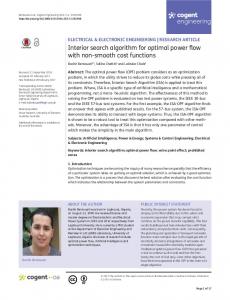
A. Application Model Many applications have data generated at multiple sites and queried by users from multiple sites. Storing all the data at a central site is impractical. Replication of data on multiple storage arrays with distant locations is necessary since multiserver retrieval can be used and the load can be distributed among the servers. An example model is provided in Figure 1, where geographically distant storage arrays are connected over a dedicated network.

B. Maximum Flow Problem Maximum flow is a general technique used in optimal response time retrieval problems [12], [18], [45]. In the maximum flow problem, the goal is to send as much flow as possible between two vertices, subject to edge capacity limits. An instance of the maximum flow problem is a network G = (V, E, s, t, u), where s ∈ V is a distinguished vertex called the source, t ∈ V is a distinguished vertex called the sink, and u is a capacity function. A flow is a pseudoflow that satisfies the flow conservation constraints: 

SSD Storage Array

HDD Storage Array

Dedicated Network

∀v ∈ V − {s, t} :

f (v, w) = 0

(1)

w∈V :(v,w)∈E

Equation 1 states that for all vertices except the source and sink, the net flow leaving that vertex is zero. The value of a flow f is the net flow into the sink as in Equation 2. 

Hybrid Storage Array

Fig. 1.

|f | =

Storage arrays connected with a dedicated network

f (v, t)

(2)

v∈V :(v,t)∈E

The maximum flow problem has been studied for over fifty years. It has a wide range of applications including the transshipment and assignment problems. Known solutions to this problem include Ford-Fulkerson augmenting path method [24], [25], the closely related blocking flow method [22], [33], network simplex method [21], [32], and push-relabel method of Goldberg and Tarjan [29]. 1) Ford-Fulkerson Method: The motivation behind the Ford-Fulkerson augmenting path method is as follows: An augmenting path is a residual s-t path. If there exists an augmenting path in Gf , then we can improve f by sending flow along this path. Ford and Fulkerson [24] showed that the converse is also true. Theorem 1: A flow f is a maximum flow if and only if Gf has no augmenting paths. This theorem motivates the augmenting path algorithm of Ford and Fulkerson’s [24], which repeatedly sends flow along augmenting paths, until no such paths remain. 2) Push-relabel Method: Push-relabel methods send flow along individual edges instead of entire augmenting paths. This leads to better performance both in theory and practice [29]. The push-relabel algorithm works with preflows, which is a flow that satisfies capacity constraints except additional flows into a vertex is allowed called excess. A vertex with positive excess is said to be active. Each vertex is assigned a height, where initially all the heights are zero except height[s] = |V |. An iteration of the algorithm consists of selecting an active vertex, and attempting to push its excess to its neighbors with lower heights. If no such edge exists, the vertex’s height is increased by 1. The algorithm terminates when there are no more active vertices with label less than |V |.

Although traditional HDD (Hard Disk Drive) based storage arrays still dominate the market share, SSD (Solid-state Drive) based storage arrays [4], [6], [7], [9] and hybrid storage arrays [3], [5], [8], [10] composed of SSDs and HDDs gain a lot of attention recently. Our model supports the heterogeneity of the storage arrays such that they can be HDD based, SSD based or hybrid. In addition to the heterogeneity of the storage arrays, we also consider the network delay to the storage arrays and the initial load of the disks caused by the previous queries. Many Internet service providers now offer dedicated Internet access with bandwidth, latency, packet loss, and availability guarantees. For example, XO communications’ dedicated Internet access [1] guarantees round-trip latency of 65 milliseconds edge-to-edge within the XO network, roundtrip packet loss of at most 1%, and availability of 100%. Using the guarantees given by a dedicated network, an estimate network delay to a storage array can be determined. Besides the network delay, initial loads of the disks from the previous queries can also be calculated easily since it is based on how the previous queries are scheduled. Potential applications of the model are as follows: • Dataset for an application is stored on a storage array. A new high-end storage array is purchased. Instead of moving all the data to the new storage array, a system spanning the two storage arrays can be used. Storage arrays are costly and making the most out of them is crucial. • A large dataset is split and stored at storage arrays at multiple sites. We want to run an application that potentially processes parts of the whole dataset. The model above allows us to do this efficiently. • High-end computer centers with storage arrays can be combined to create storage systems with much larger capacity in an affordable way. • An SSD based or hybrid storage array is added to a

C. Replicated Declustering and Retrieval A replicated declustering of 7 × 7 grid using 7 disks is given in Figure 2. The grid on the left represents the first copy and the grid on the right represents the second copy.

12

the sink have capacity 1. The capacity of the edges between the disks and the sink are set to  |Q| N .

Each square denotes a bucket and the number on the square denotes the disk that the bucket is stored at. An i × j range query has i rows and j columns. For retrieval of an i × j range query from homogeneous disks, the best we can expect is  i∗j 7  disk accesses and this happens if the buckets of the query are spread to the disks in a balanced way. In most cases, this is not possible without replication. q1 q1 5 1 4

6

4 0

2 3 5 6 1 2

2 5

0 3

1 4

2 5

3 6

4 5 0 1

6 2

0

1 4

2

3

5 1 4

6

3 4 6 0

0 3 6

0

2 5 1

Fig. 2.

3

0

1 2 2 3 4

3 4 5 6 5 6 0 1

4

5 6

0 1

2 3

6 1

0 1 2 3 2 3 4 5

4 5 6 0

3 5

4 5 6 0

BUCKETS [0,0] [0,1]

s

[1,0] [1,1] [2,0] [2,1]

6 0 1 2 1 2 3 4

Fig. 3.

Orthogonal Allocation

DISKS 0 1 2 3

t

4 5 6

Max-flow representation of query q1 for single site

Maximum flow representation of query q1 for single site is given in Figure 3. Maximum flow is shown using thick lines in the figure. Since query q1 has only 6 buckets and  67  = 1, all the edges have capacity 1 in this case. When using maximum flow representation, if the maximum flow between the source and the sink is |Q|, then the query can be retrieved using  |Q| N  disk accesses. Otherwise, we need to increment the capacities of all the edges going to the sink by one and re-run the maxflow algorithm. We repeat this incrementation process until the flow of |Q| is reached. Max-flow algorithm is called O(|Q|) time in the worst case where all the buckets are stored at a single disk.

The notation used in this paper along with their meanings is given in Table I. TABLE I N OTATION Notation Meaning N Total number of disks in the system |Q| Total number of buckets to be retrieved; query size c Number of copies for each bucket Cj Average retrieval cost of a single bucket from disk j Dj Network delay to the server where disk j is located Xj Time it takes for disk j to be idle if busy, 0 otherwise

D. Basic Retrieval Problem In optimal response time retrieval problem, we have N disks and |Q| buckets. Each bucket can be replicated among multiple disks. The aim is to find a way of retrieving the requested buckets of a query from the disks so that the overall response time of the query is minimized. The basic problem assumes that the disks are homogeneous without having any initial load or network delay and they are all located on a single site. In this case, the overall response time of the query is determined by the disk that is used to retrieve the maximum amount of buckets. In other words, we need to retrieve as few buckets as possible from the disk that is used to retrieve the maximum amount of buckets. Basic problem is solved as a max-flow problem using graph theory. When replication is used, each bucket is stored on multiple disks and we have to choose one of the disks for retrieval of the bucket. Consider the query q1 given in Figure 2. Query q1 is a 3 × 2 query with optimal retrieval cost of  3×2 7  = 1. However, since in the first copy the buckets [0, 0] and [2, 1] are both stored on disk 0, retrieval using the first copy requires 2 disk accesses. When we consider both copies, we can represent the problem as a maximum flow problem [18] as in Figure 3. For each bucket and for each disk we create a vertex. In addition, two more vertices called source and sink are created. Source vertex s is connected to all the vertices denoting the buckets and all the vertices denoting the disks are connected to the sink vertex t. An edge is created between vertex vi denoting bucket i and vertex vj denoting disk j if bucket i is stored on disk j. Next step is to set the capacities of the edges. All the edges except the ones between the disks and

E. Generalized Retrieval Problem Besides covering the properties of the basic problem, generalized retrieval problem also handles the heterogeneity of the disks, initial loads, multi-site retrieval, and network delay. Consider the query q1 given in Figure 2 again but this time assume that the grid on the left represents the allocation at site 1 and the grid on the right represents the allocation at site 2. There are 14 disks in the system, disks 0-6 are located at site 1 and the disks 7-13 are located at site 2. Generalized retrieval problem can be formulated as a maximum flow problem [12]. For the set of parameters summarized in Table II, optimal response time retrieval of the query q1 is shown in Figure 4 using the thick lines. Let E be the edge set holding every edge ej between the disk vertex j and the sink. As in the basic problem, all the edges except the ones in E have capacity 1. In the basic problem, since all the disks are homogeneous without having any network delay or initial load, it is possible to initially set the capacities of all the edges in E to the theoretical lower bound  |Q| N . If the flow of |Q| cannot be reached, capacities of the edges is E are incremented all at the same time. However, this is not possible for the generalized retrieval problem since different disks might have different retrieval costs depending on their speed, initial load, and network delay. Figure 4 shows the proper values of the capacities for the parameters defined in in Table II. In order to set the capacities of the edges in E properly, [12] proposes a binary capacity scaling algorithm. The algorithm defines a range where the optimal response time is known to

13

TABLE II S YSTEM PARAMETERS Disk j Cj (ms) Dj (ms) Xj (ms) 0-6 8.3 2 1 7,8,10,13 6.1 1 0 9,11,12 13.2 1 0 BUCKETS

Algorithm 1 F ordF ulkersonBasic() 1: for all e ∈ E do |Q| 2: caps[e] ←  N  3: for i ← 1 to |Q| do 4: df s success = DF S(G, v[i], t, caps, f low, path) 5: while (!df s success) do 6: for all e ∈ E do 7: caps[e]++ 8: df s success = DF S(G, v[i], t, caps, f low, path) 9: for all e ∈ path do 10: if target(e) =  t then 11: G.reverse edge(e) 12: if isDirectionReverse(e) then 13: f low[e]- 14: else 15: f low[e]++ 16: f ixReversedEdges()

DISKS 0 1 2 3

[0,0]

4

[0,1]

5

[1,0]

6

s [1,1]

7

[2,0]

8

[2,1]

9 10

1 1 0 1 1 0 1 1 1 0 1 0 0 0

t

Algorithm 2 F ordF ulkersonIncremental() 1: for all e ∈ E do 2: caps[e] ← 0 3: for i ← 1 to |Q| do 4: df s success = DF S(G, v[i], t, caps, f low, path) 5: while (!df s success) do 6: IncrementM inCost() 7: df s success = DF S(G, v[i], t, caps, f low, path) 8: for all e ∈ path do 9: if target(e) = t then 10: G.reverse edge(e) 11: if isReverse(e) then 12: f low[e]- 13: else 14: f low[e]++ 15: f ixReversedEdges()

11 12 13

Fig. 4.

Max-flow representation of query q1 for 2 sites

be within this range. In each iteration, the algorithm picks the middle value of this range, calculates the capacities for this middle value and runs the maximum flow algorithm. Depending on the flow value, the algorithm decreases the range by half either eliminating the top range or the bottom range. After the range is small enough, the algorithm reaches to the optimal response time retrieval by incrementing the capacity of the edge yielding the minimum cost and running the max-flow in each iteration. The algorithm terminates when the maximum flow of |Q| is reached. Readers are directed to [12] for more details. The problem with the solution proposed in [12] is that it uses maximum flow as a black box technique. Therefore, in each run of the maximum flow with different capacities, flow values are calculated starting from zero all over again. Since the algorithm increments the capacities used in one previous run for each step, current run of maximum flow can start from the flow values calculated in the previous run. This approach will obviously save considerable amount of maximum flow calculations; however, it requires an integrated maximum flow solution for the generalized retrieval problem.

Algorithm 3 IncrementM inCost() 1: min cost ← M AXDOU BLE 2: for all e ∈ E do 3: v ← G.source(e) 4: if G.in degree(v) ≤ caps[e] then 5: E.delete(e) 6: else 7: cost[e] ← D[e] + X[e] + (caps[e] + 1) ∗ C[e] 8: if costs[e] < min cost then 9: min cost ← costs[e] 10: for all e ∈ E do 11: if costs[e] == min cost then 12: caps[e]++

no augmenting path exists, capacities of the edges in E are incremented by one until a path is found through the lines 5-8. For each edge in the path, line 11 reverses its direction if the edge is between a bucket vertex and a disk vertex. This reversal is necessary to be able to change the retrieval decision of a previously assigned bucket. Finally, lines 12-15 increments or decrements the flow of each edge in the path depending on its direction. If the edge direction is not its original direction, then the flow is decremented meaning that the retrieval choice is changed, otherwise the flow is incremented. At the end of the algorithm, we have to fix the directions of the edges since some of them might have a reverse direction. It is proven in [18] that Algorithm 1 has the worst case complexity of O(c ∗ |Q|2 ) since the DFS might try c ∗ |Q| edges in the worst case. Note that the capacity incrementation in lines 6-7 is performed at

III. F ORD -F ULKERSON BASED S OLUTION The first integrated algorithm we propose for the generalized retrieval problem uses the Ford-Fulkerson method. Algorithm 1 shows a Ford-Fulkerson based integrated algorithm proposed in [18] for the basic retrieval problem. Algorithm 1 assumes that flow values of the edges going out of the source vertex are all initialized to 1 at the beginning. Lines 1-2 sets the capacities of the edges in E to the theoretical lower bound  |Q| N , where E holds all the edges between the disk vertices and the sink. Then, for each bucket i in the query, the algorithm searches for an augmenting path from the vertex representing the bucket i to the sink vertex in lines 3-4. If

14

problem. Similar to Algorithm 2, Algorithm 5 increments the capacity of the edge yielding the minimum retrieval cost in each incrementation step as in line 2 and runs until the excess value of the sink reaches to |Q|. For every iteration, we clear the queue as in line 3 and initialize the height values as in line 11-13. Push-relabel operations ensure that excess values of the vertices except the source and the sink vertex are all 0 when the algorithm terminates. Therefore, we only set the excess value of source to 0 in every iteration as in line 14. Note that our aim is conserving the flows found in the previous runs, therefore flow values are not initialized back to 0. In addition to this, the algorithm should add vertices to the queue only if they can pass more flow in the next push/relabel operations. We check this by using the δ value calculated in line 6 and initialize these vertices only in lines 7-10.

most O(|Q|) time during the entire execution of the algorithm. Algorithm 1 works for the basic retrieval problem only. In order to extend this algorithm to the generalized retrieval problem, we propose Algorithm 2. Algorithm 2 starts to the capacity incrementation from 0 (lines 1-2) since is not possible to use a simple formula like  |Q| N  as a lower bound in the generalized case. Secondly, since each disk might have a different retrieval cost, capacities of the edges in E cannot be incremented at the same time. Only the capacity of the edge yielding the minimum retrieval cost should be incremented in each incrementation step. Algorithm 2 calls Algorithm 3 for this purpose in line 6, which is the main difference between Algorithm 2 and Algorithm 1. Algorithm 3 determines the edges in E yielding the minimum retrieval cost in lines 7-9 and increments the capacities of the edges with this minimum cost in lines 11-12. Note that, if there are more than one edges yielding the same retrieval cost, their capacities are incremented at the same time as in the basic problem. Lines 3-5 remove the edge from the edge set E if the disk associated with that edge cannot be used to retrieve any more buckets. This removal ensures that the number of incrementation steps are bounded by O(c ∗ |Q|) in the worst case. Therefore, worst case complexity of the Algorithm 2 is O(c2 ∗ |Q|2 ).

Algorithm 5 P ushRelabelIncremental() 1: while excess[t] = |Q| do 2: IncrementM inCost() 3: QU EU E.clear() 4: for all out edges(e,s) do 5: v ← target(e) 6: δ ← cap[e] − f low[e] 7: if d > 0 then 8: QU EU E.append(v) 9: f low[e] ← cap[e] 10: excess[v] += cap[e] 11: for all nodes(v,G) do 12: height[v] ← 0 13: height[s] ← G.number of nodes() 14: excess[s] ← 0 15: while QU EU E = ∅ do 16: apply push/relabel operations by updating the QU EU E 17: return excess[t]

IV. P USH - RELABEL BASED S OLUTION Although Ford-Fulkerson based algorithms are simple and easy to implement, most of the practical maximum flow implementations are based on push-relabel based algorithms. Therefore, we also propose a push-relabel based integrated maximum flow algorithm for the generalized optimal response time retrieval problem. Algorithm 4 presents a basic pushrelabel based maximum flow algorithm. Lines 1-8 show the initialization step. Push/relabel operations of the algorithm are performed in lines 9-10, which we skip for the sake of simplicity; however, readers are directed to [29] for more details. When the algorithm terminates, excess value of the sink holds the maximum flow amount that can be pushed from the source s to the sink t. Our implementation of Algorithm 4 has the complexity of O(|V 3 |), where |V | is the number of vertices in G. This is possible since we use the FIFO ordering for selecting vertices and exact height calculation heuristics suggested by [19].

Algorithm 5 solves the generalized optimal response time retrieval problem using an integrated push-relabel based maximum flow algorithm. Although we can conserve the flows calculated for the previous capacities in the current run, the algorithm still considers all possible retrieval times starting from the minimum in an exhaustive search manner. Since the graph has |V | = |Q| + N + 2 vertices, Algorithm 5 has the worst case complexity of O(c ∗ |Q|4 ) where O(|Q|3 ) comes from the push/relabel operations (assuming |Q| > N ) and O(c ∗ |Q|) comes from IncrementM inCost(). Since we are conserving the flows, the algorithm is expected to run faster in practice; however, we can still improve the worst case complexity further by using the binary capacity scaling technique presented in [12]. Binary capacity scaling technique will bring the capacity values up to an initial value in O(log(|Q|)) operations before the incrementation step is started by Algorithm 5. By this way, number of incrementation steps will be bounded by N , the number of disks in the system. Algorithm 6 presents our final push-relabel based integrated maximum flow algorithm that uses the binary capacity scaling technique. First, we define a range [tmax , tmin ) in lines 111 where we know the optimal response time retrieval lies within. In order to ensure this, we calculate tmax assuming that all the query buckets are retrieved from the disk with the largest retrieval cost, and tmin assuming that all the query

Algorithm 4 P ushRelabelBasic() 1: 2: 3: 4: 5: 6: 7: 8: 9: 10: 11:

for all out edges(e,s) do v ← target(e) QU EU E.append(v) f low[e] ← cap[e] excess[v] += cap[e] for all nodes(v,G) do height[v] ← 0 height[s] ← G.number of nodes() while QU EU E = ∅ do apply push/relabel operations by updating the QU EU E return excess[t]

Algorithm 5 presents a push-relabel based integrated maximum flow algorithm for the generalized response time retrieval

15

V. PARALLEL P USH - RELABEL I MPLEMENTATION

buckets are retrieved from the disk with the smallest retrieval cost. Since we want to ensure that there is no solution for tmin , we subtract the min speed value from tmin in line 11. min speed is the average retrieval time of a single block from the fastest disk in the system calculated in lines 9-10.

Most new generation storage arrays are powered with multicore processors. Since retrieval decision is a time critical issue, it is reasonable to use multi-threaded implementations in order to reduce the execution time of retrieval algorithms further. Many push-relabel based parallel maximum flow algorithms are proposed in the literature such as [13] and [14]. However, both of these implementations require locks to perform push/relabel operations. Since locks are known to have expensive overheads [20], we decided to use the asynchronous parallelization method presented in [31]. The algorithm presented in [31] uses the same push/relabel techniques proposed in [29]; however, it does not require any locks or barriers to protect the push/relabel operations. Instead, they use atomic read-modify-write instructions. We implemented a parallel version of our Algorithm 6 using pthreads and the techniques described in [31]. Since the parallelization should take place in the push/relabel operations, line 29 of the Algorithm 6 is modified to support multi-threaded push/relabel operations as it is described in [31].

Algorithm 6 P ushRelabelBinary() 1: 2: 3: 4: 5: 6: 7: 8: 9: 10: 11: 12: 13: 14: 15: 16: 17: 18: 19: 20: 21: 22: 23: 24: 25: 26: 27: 28: 29: 30: 31: 32: 33: 34: 35: 36: 37: 38: 39: 40: 41: 42:

min speed ← M AXDOU BLE tmin ← M AXDOU BLE tmax ← 0 for all e ∈ E do if D[e] + X[e] + |Q| ∗ C[e] > tmax then tmax ← D[e] + X[e] + |Q| ∗ C[e]  ∗ C[e] < tmin then if D[e] + X[e] +  |Q| N tmin ← D[e] + X[e] +  |Q|  ∗ C[e] N if C[e] < min speed then min speed ← C[e] tmin -= min speed while (tmax − tmin ) ≥ min speed do tmid ← tmin + (tmax − tmin ) ∗ 0.5 for all e ∈ E do caps[e] ← (tmid − D[e] − X[e])/C[e] QU EU E.clear() for all out edges(e,s) do v ← target(e) δ ← cap[e] − f low[e] if d > 0 then QU EU E.append(v) f low[e] ← cap[e] excess[v] += cap[e] for all nodes(v,G) do height[v] ← 0 height[s] ← G.number of nodes() excess[s] ← 0 while QU EU E = ∅ do apply push/relabel operations by updating the QU EU E if excess[t] = |Q then StoreF lows() tmp excess t ← excess[t] tmin ← tmid else RestoreF lows() excess[t] ← tmp excess t tmax ← tmid RestoreF lows() excess[t] ← tmp excess t for all e ∈ E do caps[e] ← (tmin − D[e] − X[e])/C[e] P ushRelabelIncremental()

VI. E XPERIMENTAL R ESULTS In this section, we provide experimental results using various sets of parameters. Our aim is comparing the execution times (running time, runtime) of the proposed algorithms with the existing ones. We investigate the impact of allocation scheme, query type, query load, disk speed, network delay to the site, and initial load of the disks on the execution times. We implemented the experiments in C++ and compiled using g++ version 4.4.3 optimization level 1 (-O1) using the graph structure of LEDA [34] except the parallel implementation. For the parallel generalized retrieval algorithm, we used C and the pthread library in order to comply with the original implementation presented in [31]. Parallel implementation is compiled using gcc version 4.4.3 optimization level 3 (-O3) as in [31]. The machine we used has dual Intel Xeon X5672 quad-core processors with total of 8 cores. Each core has 3.2 GHz of clock speed and the machine has 32GB of physical memory running on an Ubuntu 10.04.03 LTS operating system.

Algorithm 6 finds the capacities of the flow graph for tmid in line 15, performs initialization of the push/relabel operations through the lines 16-27, and applies push/relabel operations in lines 28-29. If there is no solution such that excess[t] = |Q|, we store the current flow state of the graph as in lines 31-32 to be used later to eliminate unnecessary flow calculations. Also, we increase tmin to tmid as in line 33 to reduce the range. If there is a solution such that excess[t] = |Q|, since we cannot be sure of the optimality of the solution, we restore the saved flow values and decrease tmax to tmid as in lines 35-37. The algorithm stops when the range is smaller than min speed, restores the saved flows, calculates the final capacities using tmin , and calls P ushRelabelIncremental() through the lines 38-42. Worst case complexity of the Algorithm 6 is O(log(|Q|) ∗ |Q|3 ); however, it is expected to perform better in practice thanks to the flow conservation property.

A. Allocation Scheme We have experimental results for three different allocation schemes described below. • Random Duplicate Allocation: Random Duplicate Allocation (RDA) [38] stores a bucket on two disks chosen randomly from the set of disks. Retrieval cost of random allocation is at most 1 more than the optimal with high probability for single site retrieval [38]. • Orthogonal Allocation: Orthogonal allocations [23], [39] guarantee that when the disks that a bucket is stored at is considered as a pair, each pair appears only once in the disk allocation. In an N × N declustering system with N disks, there are N 2 buckets and N 2 pairs. So, it is possible to have each pair exactly once. For the first copy, we used the threshold based declustering scheme [44].

16

•

Dependent Periodic Allocation: A d-dimensional disk allocation scheme f (i1 , i2 , . . . , id ) is periodic if f (i1 , i2 , . . . , id ) = (a1 ∗i1 +a2 ∗i2 +. . .+ad ∗id) mod N , where N is the number of disks and each ai i = 1 . . . d satisfies gcd(ai , N ) = 1 and ai = 0 [11], [46]. For the first copy, we use the allocation scheme yielding the lowest additive error based on the results provided in [11]. For the second copy, a shifted version of the first copy is used. The two allocations are in the form of f (i, j) = a1 ∗ i + a2 ∗ j mod N and g(i, j) = f (i, j) + m mod N, 1 ≤ m ≤ N − 1.

provided in the table is the average access time to read a block in our system, which is calculated using the Ubuntu disk utility benchmark. Average access time of a block is defined as the summation of spin-up time, seek time, rotational latency and transfer time for HDDs; just transfer time for SSDs. Producer Seagate WD Seagate OCZ Intel

B. Query Types

TABLE III D ISK S PECIFICATIONS Model Type RPM Barracuda HDD 7.2K Raptor HDD 10K Cheetah HDD 15K Vertex SSD X25-E SSD -

Time (ms) 13.2 8.3 6.1 0.5 0.2

E. Experiment Parameters

We have experimental results for two different types of queries; range queries and arbitrary queries. • Range Query: Range queries are rectangular in shape. We assume a wraparound grid consistent with the choice of disk allocations. A range query is identified with 4 parameters (i, j, r, c) 0 ≤ i, j ≤ N − 1, 1 ≤ r, c ≤ N . i and j are indices of the top left corner of the query and r, c denote the number of rows and columns in the query. The number of distinct range queries on an N ×N +1) 2 grid is ( N ∗(N ) , which can be found by counting the 2 number of ways to choose two points out of N + 1 row  and column points on the grid as follows: N2+1 ∗ N2+1 . • Arbitrary Query: Arbitrary queries have no geometric shape. Any subset of the set of buckets is an arbitrary query. We can denote arbitrary queries as a set and the N 2  2  number of arbitrary queries is i=1 Ni which is equal 2 to 2N (number of subsets of a set with N 2 elements).

All the experiments conducted are summarized in Table IV. Delay and initial load values are given in milliseconds. R(2,10,2) means that a number among the set 2, 4, 6, 8, and 10 is chosen randomly. If the system is homogeneous, the properties of the cheetah disk is used for all the disks in the system. If the system is heterogeneous, then the disks are chosen randomly among the disk group indicated in the table. Disk groups can be HDDs, SSDs, or HDDs+SSDs. TABLE IV E XPERIMENTS Exp. # of Disk Site 1 Site 2 Num. Sites Prop. Disks Delays Loads Disks Delays Loads 1 2 hom. cheetah 0 0 cheetah 0 0 2 2 het. ssd 0 0 hdd 0 0 3 2 het. hdd 0 0 ssd 0 0 4 2 het. ssd+hdd 0 0 ssd+hdd 0 0 5 2 het. ssd+hdd R(2,10,2) R(2,10,2) ssd+hdd R(2,10,2) R(2,10,2)

F. Results In this section, we provide some of the experimental results that are interesting for our purposes. All the results are available on the project web page [2]. In all experiments, we used an N ×N grid for N disks and for each value of N , 1000 queries are performed. For every experiment we performed, we compared the total optimal response time values of these 1000 queries for each algorithms we tested and found out that the results are matching as expected. In this paper, we are interested in the execution time comparison of the algorithms. Therefore, we do not share the response time values of the experiments. An in depth study for the effect of different parameters on the response time of the queries can be found in [12]. 1) Ford-Fulkerson vs. Push-relabel: In this section, we compare the execution times of the Ford-Fulkerson based algorithms with the Push-relabel based algorithms. Since the basic retrieval problem is a subset of the generalized retrieval problem, algorithms proposed for the generalized retrieval problem can also solve the basic retrieval problem. Experiment 1 is an example of a basic retrieval problem where the disks are homogeneous and there is no initial load or network delay. Figure 5 compares the Algorithm 1 with the Algorithm 6 using the Experiment 1, where x-axis shows the number of disks and y-axis shows execution times. Even though Ford-Fulkerson based retrieval algorithms have better worst case complexity,

C. Query Load pik

We use three different query loads.We use the notation to denote the probability that a query in load i can be retrieved in k disk accesses optimally. Once the optimal number of disk accesses k is selected, the number of buckets is selected uniformly from the range [(k − 1)N + 1, kN ]. • Load 1: The distribution of queries is similar to the distribution of queries for the particular query type. For the distribution of range queries, smaller size queries are more likely; for the distribution of arbitrary queries, medium size queries are more likely. Expected bucket 2 size of load 1 queries is N4 + O( N1 ) for range queries 2 and N2 + O( N1 ) for arbitrary queries. • Load 2: The distribution of queries is uniform. We achieve this by setting p2k = N1 . Expected bucket size 2 of load 2 queries is N2 . • Load 3: Much smaller queries than load 1 and load 2 are 2N more likely. We achieve this by setting p3k = (2N −1)∗2 k. In this case p3k = 12 p3k−1 , 2 ≤ k ≤ N . Expected bucket size of load 3 queries is 3N 2 . D. Disks We have experimental results on five different disks. Specifications of the disks are given in Table III. The time value

17

LOAD 1 - RANGE - RDA

LOAD 2 - ARBITRARY - RDA

250 200 150 100 50 0 0

10

20

30

40

50 N

60

70

80

1000 900 800 700 600 500 400 300 200 100 0

90 100

(a) Range, Load 1 Fig. 5.

10

LOAD 1 - ARBITRARY - Orthogonal

20

30

40

50 N

60

70

80

250 200 150 100 50 0 40

50

60

70

80

600

0.1 10

20

30

40

50 N

60

70

80

90 100

LOAD 3 - ARBITRARY - Orthogonal

500 400 300 200 100

90 100

Ford-Fulkerson Push-relabel

0.8 0.7 0.6 0.5 0.4 0.3 0.2 0.1 0

0

10

20

30

40

N

(a) Arbitrary, Load 1 Fig. 6.

0.2

0.9 Ford-Fulkerson Push-relabel

0 30

0.3

0

Avg. Runtime Per Query (msec)

Avg. Runtime Per Query (msec)

300

20

0.4

LOAD 2 - RANGE - Orthogonal

350

10

0.5

90 100

700

0

0.6

(b) Arbitrary, Load 2 (c) Range, Load 3 Experiment 1, RDA, Ford-Fulkerson - Push-relabel Execution Time

Ford-Fulkerson Push-relabel

400

Ford-Fulkerson Push-relabel

0.7

0 0

450 Avg. Runtime Per Query (msec)

LOAD 3 - RANGE - RDA 0.8

Ford-Fulkerson Push-relabel

Avg. Runtime Per Query (msec)

Ford-Fulkerson Push-relabel

300

Avg. Runtime Per Query (msec)

Avg. Runtime Per Query (msec)

350

50 N

60

70

80

90 100

0

10

20

30

40

50

60

70

80

90 100

N

(b) Range, Load 2 (c) Arbitrary, Load 3 Experiment 5, Orthogonal, Ford-Fulkerson - Push-relabel Execution Time

algorithm. For example, Orthogonal allocation requires more incrementation steps for the range queries and RDA requires more incrementation steps for the arbitrary queries. In these cases, integrated algorithm performs about 1.3X faster than the black box algorithm. By this way, performance gap between different allocation schemes are also decreased thanks to the integrated algorithm. This can be observed more clearly in Figure 8.

push-relabel based retrieval algorithms are better in practice. Execution time of the push-relabel based Algorithm 6 is at most 25 milliseconds for load 2 with N = 100 and |Q| = 5000; however, Ford-Fulkerson based Algorithm 1 requires almost a second for same case. The results are similar for load 1. Since the query sizes are small for load 3, Algorithm 1 is slightly better than Algorithm 6 for N < 60 (less than 0.1 milliseconds difference); however, Algorithm 1 does not scale well when the number of disks and the query size increase.

Figure 8 compares the black box and the integrated pushrelabel based retrieval algorithms using the Experiment 3. Figure 8(a) shows the execution time of the black box algorithm. Retrieval algorithm for dependent allocations have lesser execution time since their retrieval choices are more obvious than Orthogonal allocations and RDA. However, execution times for Orthogonal and RDA are expected to be similar. Figure 8(b) shows the execution time of the integrated algorithm. As it is clear from the graph, execution time for Orthogonal and RDA are similar and execution time for dependent is slightly less than the others as expected. In other words, integrated algorithm decreased the execution time gap between different allocation schemes. Therefore, execution time ratio of black box and integrated algorithm presented in Figure 8(c) is higher for the Orthogonal allocation.

Figure 6 compares the Ford-Fulkerson based Algorithm 2 with the Push-relabel based Algorithm 6 for the generalized retrieval problem of Experiment 5. Performances are similar to the basic retrieval case shown in Figure 5. For Experiment 5, push-relabel based Algorithm 6 requires at most 30 ms when N = 100 and |Q| = 5000. Figure 5 and Figure 6 clearly show that push-relabel based retrieval algorithms are superior to the Ford-Fulkerson based retrieval algorithms for both the basic retrieval problem and the generalized retrieval problem. 2) Blackbox Push-relabel vs. Integrated Push-relabel: In this section, we compare the execution time of the black box push-relabel based binary retrieval algorithm proposed in [12] with our integrated binary push-relabel algorithm presented in Algorithm 6. Black box algorithm uses LEDA’s pushrelabel implementation and the integrated algorithm modifies the same implementation for fair results. Figure 7 shows this comparison for the basic retrieval case using Experiment 1, where x-axis shows the number of disks and the y-axis shows the execution time ratios (black box/integrated). Since capacities of the disks are incremented at the same time in the basic retrieval case, less capacity incrementation steps are performed. Therefore, flow conservation property of the integrated algorithm could not be exploited. Nonetheless, if a certain allocation scheme requires more capacity incrementation, then the integrated algorithm clearly outperforms the black box

Figure 9 shows the execution time comparison of the black box and the integrated algorithm for the Experiment 5, where we see the most dramatic performance improvement of the integrated algorithm. Integrated algorithm is up to 2.5 times faster than the black box algorithm. As the number disks and the query sizes increase, performance improvement of the integrated algorithm also increases. The reason for this performance improvement lies in the flow conservation property of the integrated algorithm. Retrieval decision is harder in Experiment 5 since all the parameters are random. Therefore, Experiment 5 requires more incrementation steps

18

LOAD 1 - RANGE

LOAD 2 - ARBITRARY

Runtime Ratio (bb/int)

1.15 1.1 1.05 1

1.25 1.2 1.15 1.1 1.05 1 0.95

0.9

0.9 0

10

20

30

40

50 N

60

70

80

(a) Range, Load 1 Fig. 7.

90 100

10

LOAD 1 - RANGE - BLACK BOX

20

30

40

50 N

60

70

80

Avg. Runtime Per Query (msec)

15 10 5 0

0

30

40

50

60

70

80

10

20

30

40

50 N

60

70

80

90 100

70

80

90 100

LOAD 1 - RANGE 1.9

RDA Dependent Orthogonal

16 14

90 100

RDA Dependent Orthogonal

1.8

12 10 8 6 4

1.7 1.6 1.5 1.4 1.3 1.2

2 0

20

1 0.95

LOAD 1 - RANGE - INTEGRATED

20

10

1.1 1.05

90 100

18 RDA Dependent Orthogonal

0

1.15

(b) Arbitrary, Load 2 (c) Range, Load 3 Experiment 1, Push-relabel, Black Box/Integrated Execution Time Ratio

30 25

RDA Dependent Orthogonal

0.9 0

Runtime Ratio (bb/int)

Runtime Ratio (bb/int)

1.2

1.2 RDA Dependent Orthogonal

1.3

0.95

Avg. Runtime Per Query (msec)

LOAD 3 - RANGE

1.35 RDA Dependent Orthogonal

Runtime Ratio (bb/int)

1.3 1.25

1.1 0

10

20

30

40

50

N

60

70

80

90 100

0

10

20

30

40

N

50

60

N

(a) Black Box Execution Time (b) Integrated Execution Time (c) Execution Time Ratio Fig. 8. Experiment 3, Arbitrary Load 1, Push-relabel Algorithms Comparison LOAD 1 - ARBITRARY

LOAD 2 - ARBITRARY 1.9 RDA Dependent Orthogonal

2.4

2 1.8 1.6 1.4

Runtime Ratio (bb/int)

2.2

2.2 2 1.8 1.6 1.4

1.2

1.2 10

20

30

40

50

60

70

80

90 100

Fig. 9.

LOAD 1 - ARBITRARY - ORTHOGONAL - 100 Disks 1.6 1.5 1.4 1.3 1.2 1.1 1 0.9 30

40

50

1.6 1.5 1.4

10

20

30

40

50

60

70

80

90 100

0

10

20

30

40

60

70

80

50

60

70

80

90 100

N

LOAD 2 - RANGE - ORTHOGONAL - 100 Disks Running Time Ratio (parallel/single)

speed up (avg=1.2)

20

1.7

(b) Load 2 (c) Load 3 Experiment 5, Push-relabel, Black Box/Integrated Execution Time Ratio

1.7

10

1.8

N

(a) Load 1

0

RDA Dependent Orthogonal

1.3 0

N

90 100

1.8 speed up (avg=1.19) 1.6 1.4 1.2 1 0.8 0.6 0.4 0.2 0

10

20

30

Query

40

50 Query

60

70

80

LOAD 1 - ARBITRARY - RDA - 100 Disks Running Time Ratio (parallel/single)

0

Running Time Ratio (parallel/single)

LOAD 3 - ARBITRARY

2.6 RDA Dependent Orthogonal

Runtime Ratio (bb/int)

Runtime Ratio (bb/int)

2.4

90 100

1.5 speed up (avg=1.18) 1.4 1.3 1.2 1.1 1 0.9 0.8 0

10

20

30

40

50

60

70

80

90 100

Query

(a) Arbitrary, Load 1, Orthogonal (b) Range, Load 2, Orthogonal (c) Arbitrary, Load 1, RDA Fig. 10. Experiment 5, Push-relabel Parallel/Sequential Execution Time Ratio, 2 threads, 100 disks

speed-up of 1.7X (∼1.2X on average) over the sequential implementation. The fluctuation in the graph is caused by the change in the graph structure depending on the query size. For small queries of load 3 and more than two number of threads, we observed a load-balancing issue among the threads. Together with this improvement, integrated algorithm becomes 4.25X (∼3X on average) faster than the black box implementation proposed in [12].

than the other experiments. Since there is no flow conservation in the black box algorithm, each maximum flow calculation starts with zero flows. On the other hand, integrated algorithm conserves the flow values calculated in the previous run and uses them in the current run. 3) Sequential Push-relabel vs. Parallel Push-relabel: Figure 10 shows the execution time comparison of the pushrelabel based retrieval algorithm presented in Algorithm 6 with the parallel implementation of the same algorithm using Experiment 5. Since the performance of the parallel maximum flow algorithm is highly dependent on the graph structure [31], we show different queries on the x-axis and the execution time ratio (parallel/sequential) in the y-axis. Parallel algorithm is executed using two threads for 100 disks and gains a maximum

VII. C ONCLUSION In this paper, we propose integrated maximum flow algorithms for the generalized retrieval problem where heterogeneous disks with initial loads can be located on multiple sites having different network delays. Our first algorithm is

19

based on the Ford-Fulkerson method and the second algorithm is based on the Push-relabel technique. We investigate the execution time of the proposed and existing algorithms for the basic and the generalized retrieval problems. Experimental results using various replication schemes, query types, query loads, disk specifications, site delays, and initial disk loads show that proposed Push-relabel based algorithms are superior to the Ford-Fulkerson based algorithms. In addition to this, integrated push-relabel based algorithm is up to 2.5X faster than the existing black box counterpart. We also implemented a parallel version of the proposed push-relabel based integrated algorithm and observed a speed-up of 1.7X maximum (∼1.2X on average) over the sequential algorithm. Together with the parallel implementation, our proposed integrated algorithm runs up to 4.25X (∼3X on average) faster than the existing black box algorithm.

[19] Boris V. Cherkassky and Andrew V. Goldberg. On implementing pushrelabel method for the maximum flow problem. Technical report, Stanford, CA, USA, 1994. [20] David Culler, J. P. Singh, and Anoop Gupta. Parallel Computer Architecture: A Hardware/Software Approach. Morgan Kaufmann, August 1998. [21] George B. Dantzig. Application of the Simplex Method to a Transportation Problem. 1951. [22] E. A. Dinic. Algorithm for solution of a problem of maximum flow in networks with power estimation. Sov. Math. Dok, 11:1277–1280, 1970. [23] H. Ferhatosmanoglu, A. S¸. Tosun, and A. Ramachandran. Replicated declustering of spatial data. In 23rd ACM SIGMOD-SIGACT-SIGART Symposium on Principles of Database Systems, pages 125–135, June 2004. [24] L. R. Ford and D. R. Fulkerson. Maximal Flow through a Network. Canadian Journal of Mathematics, 8:399–404, 1956. [25] L. R. Ford and D. R. Fulkerson. Flows in Networks. Princeton University Press, 1962. [26] K. Frikken. Optimal distributed declustering using replication. In 10th International Conference on Database Theory (ICDT 2005), pages 144– 157, 2005. [27] K Frikken, M. Atallah, S. Prabhakar, and R. Safavi-Naini. Optimal parallel i/o for range queries through replication. In 13th International Conference on Database and Expert Systems Applications (DEXA), pages 669–678, 2002. [28] V. Gaede and O. Gunther. Multidimensional access methods. ACM Computing Surveys, 30:170–231, 1998. [29] Andrew V. Goldberg and Robert E. Tarjan. A new approach to the maximum flow problem. Journal of the ACM, 35:921–940, 1988. [30] A. Guttman. R-trees: A dynamic index structure for spatial searching. In Proc. ACM SIGMOD, pages 47–57, 1984. [31] Bo Hong and Zhengyu He. An asynchronous multithreaded algorithm for the maximum network flow problem with nonblocking global relabeling heuristic. Parallel and Distributed Systems, IEEE Transactions on, 22(6):1025 –1033, june 2011. [32] P.A. Jensen and J.W. Barnes. Network flow programming. Board of advisors, engineering. Wiley, 1980. [33] A. V. Karzanov. Determining the maximal flow in a network by the method of preows. Sov. Math. Dok, 15:434–437, 1974. [34] Kurt Mehlhorn and Stefan N¨aher. Leda: a platform for combinatorial and geometric computing. Commun. ACM, 38(1):96–102, 1995. [35] K. Yasin Oktay, Ata Turk, and Cevdet Aykanat. Selective replicated declustering for arbitrary queries. In Proceedings of the 15th International Euro-Par Conference on Parallel Processing, Euro-Par ’09, pages 375–386, Berlin, Heidelberg, 2009. Springer-Verlag. [36] S. Prabhakar, K. Abdel-Ghaffar, D. Agrawal, and A. El Abbadi. Cyclic allocation of two-dimensional data. In ICDE, pages 94–101, Orlando, Florida, 1998. [37] H. Samet. The Design and Analysis of Spatial Structures. Addison Wesley, Massachusetts, 1989. [38] P. Sanders, S. Egner, and K. Korst. Fast concurrent access to parallel disks. In 11th ACM-SIAM Symposium on Discrete Algorithms, 2000. [39] A. S¸. Tosun. Replicated declustering for arbitrary queries. In 19th ACM Symposium on Applied Computing, pages 748–753, March 2004. [40] A. S¸. Tosun. Constrained declustering. In International Conference on Information Technology Coding and Computing, pages 232–237, April 2005. [41] A. S¸. Tosun. Design theoretic approach to replicated declustering. In International Conference on Information Technology Coding and Computing, pages 226–231, April 2005. [42] A. S¸. Tosun. Threshold based declustering in high dimensions. In International Conference on Database and Expert Systems Applications, pages 818–827, August 2005. [43] A. S¸. Tosun. Analysis and comparison of replicated declustering schemes. IEEE Transactions on Parallel and Distributed Systems, 18(11):1578–1591, November 2007. [44] A. S¸. Tosun. Threshold-based declustering. Information Sciences, 177(5):1309–1331, 2007. [45] A. S¸. Tosun. Multi-site retrieval of declustered data. In 28th International Conference on Distributed Computing Systems. ICDCS ’08, pages 486 –493, june 2008. [46] A. S¸. Tosun and H. Ferhatosmanoglu. Optimal parallel I/O using replication. In Proceedings of International Workshops on Parallel Processing (ICPP), pages 506–513, Vancouver, Canada, August 2002.

VIII. ACKNOWLEDGMENTS This work is partially supported by Army Research Office (ARO) Grant W911NF-11-1-0170. R EFERENCES [1] Dedicated internet access overview. http://www.xo.com/services/ network/dia/Pages/overview.aspx. XO Communications, LLC. [2] Project webpage. http://gozde.cs.utsa.edu/integrated. [3] Sun storage 7000 unified storage systems family. http://www.oracle. com/us/products/servers-storage/039224.pdf, 2009. Oracle, Inc. [4] Sun storage f5100 flash array. http://www.oracle.com/us/043970.pdf, 2009. Oracle Datasheet. Available online (6 pages). [5] Adaptec high-performance hybrid arrays (hphas). http://www.adaptec. com/nr/rdonlyres/a1c72763-e3b9-45f7-b871-a490c29a9b11/0/hpha5 fb.pdf, 2010. PMC-Sierra, Inc. [6] Nimbus data s-class enterprise flash storage systems. http://www. nimbusdata.com/products/Nimbus S-class Datasheet.pdf, 2010. [7] Ramsan-630 flash solid state disk. http://www.ramsan.com/files/ download/212, August 2010. Texas Memory Systems White Paper. [8] Equallogic ps6100xs hybrid storage array. http://www.equallogic.com/ products/default.aspx?id=10653, 2011. Dell, Inc. [9] Violin 6000 flash memory array. http://www.violin-memory.com/assets/ Violin Datasheet 6000.pdf?d=1, 2011. Violin 6000 Memory Datasheet. [10] Zebi hybrid storage array. http://tegile.biz/wp-content/uploads/2012/01/ Zebi-White-Paper-012612-Final.pdf, 2012. Tegile Systems, Inc. [11] Nihat Altiparmak and A. S¸. Tosun. Equivalent disk allocations. IEEE Transactions on Parallel and Distributed Systems, 23(3):538–546, March 2012. [12] Nihat Altiparmak and A. S¸. Tosun. Generalized optimal response time retrieval of replicated data from storage arrays. http://gozde.cs.utsa.edu/ TR1.pdf, 2012. Technical Report. [13] Richard J. Anderson and Jo˜ao C. Setubal. On the parallel implementation of goldberg’s maximum flow algorithm. In Proceedings of the fourth annual ACM symposium on Parallel algorithms and architectures, SPAA ’92, pages 168–177, New York, NY, USA, 1992. ACM. [14] David A. Bader and Vipin Sachdeva. A cache-aware parallel implementation of the push-relabel network flow algorithm and experimental evaluation of the gap relabeling heuristic. In ISCA PDCS, pages 41–48, 2005. [15] C.-M. Chen, R. Bhatia, and R. Sinha. Declustering using golden ratio sequences. In ICDE, pages 271–280, San Diego, California, Feb 2000. [16] C-M Chen and C. Cheng. Replication and retrieval strategies of multidimensional data on parallel disks. In Conference on Information and Knowledge Management (CIKM 2003), November 2003. [17] C.-M. Chen and C. T. Cheng. From discrepancy to declustering: Near optimal multidimensional declustering strategies for range queries. In Proc. ACM PODS, pages 29–38, Wisconsin, Madison, 2002. [18] L. T. Chen and D. Rotem. Optimal response time retrieval of replicated data. In ACM SIGACT-SIGMOD-SIGART Symposium on Principles of Database Systems, pages 36–44, 1994.

20