6 - MODEL TOOLS FOR IRRIGATION SCHEDULING SIMULATION: WINISAREG AND GISAREG
P. S. Fortes 1 , P. R. Teodoro1, A. A. Campos1, P. M. Mateus1, L. S. Pereira1
Abstract: ISAREG is a conceptual non-distributed water balance model for simulating crop irrigation schedules at field level and to compute irrigation requirements under optimal and/or water stressed conditions. WINISAREG is a Windows version of the model and includes two support programs, one for creating appropriate crop data inputs, KCISA, the other to compute the reference evapotranspiration, EVAP56. GISAREG is a Geographical Information System (GIS) based application integrating both ISAREG and KCISA, which was developed for application in the Aral Sea basin to support implementation of improved farm irrigation management. The integration concerns the creation of spatial and weather data bases, the models operation for different water management scenarios, and the production of crop irrigation maps and time dependent irrigation depths at selected aggregation modes. The resulting information on alternative irrigation schedules is therefore spatially distributed and shall be used to identify practices that lead to water saving and provide for salinity control. The paper includes brief descriptions of WINISAREG and GISAREG as well as on the databases and models integration and use. Keywords: Soil water balance, crop irrigation requirements, irrigation scheduling, water savings, GIS.
Introduction The irrigation scheduling simulation model ISAREG is after long in use in several parts of the World for evaluating current irrigation schedules, selecting the most appropriate irrigation scheduling for several crops, and for computing
Agricultural Engineering Research Center, Institute of Agronomy, Technical University of Lisbon, Portugal, Email:
[email protected] 1
81
P. S. Fortes, P. R. Teodoro, A. A. Campos, P. M. Mateus, L. S. Pereira
crop irrigation requirements using weather data time series (Teixeira and Pereira, 1992, Liu et al. 1998). KCISA (Rodrigues et al., 2000) was later developed and incorporated in the model to create the appropriate crop data inputs for ISAREG using the recent FAO methodology on crop evapotranspiration (Allen et al., 1998). Reference evapotranspiration is computed with EVAP56 relative to the FAO Penman-Monteith method (Allen et al., 1998). WINISAREG is a version of this model for Windows that integrates ISAREG with KCISA and EVAP56 (Pereira et al., 2003) and was more recently developed, namely for application in Central Asia. A main feature of the model is its capability to simulate alternative irrigation schedules relative to different levels of allowed crop water stress as well as to various constraints in water availability. The irrigation scheduling alternatives are evaluated from the relative yield loss produced when crop evapotranspiration is below its potential level. Examples of those successful applications to are presented by Oweis et al. (2003) and Zairi et al. (2003) for surface irrigation in the Mediterranean region. WINISAREG also includes the option to compute the groundwater contribution with a parametric function (Liu et al., 2001) which was successfully tested in Central Asia (Cholpankulov et al., 2005). Applications of WINISAREG are described by these authors. When the computation procedure is applied at the region scale it becomes heavy and slow due to the need to consider a large number of combinations of field and crop characteristics to be aggregated at sector or project scales. However, the spatially distributed characteristics of the input data required by ISAREG and KCISA makes their integration with a Geographical Information System (GIS) particularly attractive and useful. Hence, assuming that each field is homogeneous, it is possible to automatically call the model for each cropped field represented in the GIS crop fields theme and then up-scaling the results produced using a variety of attributes (Fortes et al., 2005). This is the basic procedure adopted in GISAREG, which is the GIS version of the ISAREG model. The GISAREG application was developed in the framework of this research project. The specific objectives consist of the computation of the spatially distributed crop irrigation requirements; supporting information for farmers and managers relative to alternative water saving irrigation scheduling practices, and the simulation of the demand aggregated at the main nodes of irrigation distribution systems (Fortes et al., 2005).
Model description The ISAREG model is an irrigation scheduling simulation model that performs the soil water balance at field level as described by Teixeira and Pereira (1992) and by Liu et al. (1998). The water balance is performed for a multilayered soil and follows the classical approach referred by Doorenbos and 82
Model tools for irrigation scheduling simulation
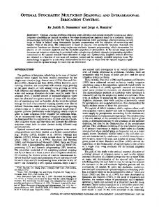
Pruitt (1977). Various times step computations are adopted, from daily up to monthly, depending on weather data availability. Inputs are precipitation, potential groundwater contribution, reference evapotranspiration (ETo), total and readily available soil water, soil water content at planting and crop factors relative to crop growth stages, crop coefficients, root depths and water-yield response factor (Fig. 1). The model input data can be provided at run-time by keyboard or trough pre-defined ASCII Files.
Soil and crop data
Program KCISA
Model ISAREG
U2
Soil
WaterRestr.
GW
Irrigation management
Pe
Irrig. Options
Crop
ETo
Agronomic data
Program EVAP56
RHmin or Tmax, T min)
Meteorológical data
Tmax Tmin RH Rs or n U2
ISAREG
SOIL WATER BALANCE
Searching an
Computing
irrigation
crop irrigation
schedule
requirements
Evaluation of an irrigation schedule
Fig. 1. Diagram of ISAREG model and links with programs KCISA and EVAP56.
The ISAREG model performs the irrigation scheduling simulations according to user-defined options such as: • •
•
to define an irrigation scheduling to maximize crop yields, i.e. without crop water stress; to define an irrigation scheduling using selected irrigation thresholds, including for allowed water stress and responding to water restrictions imposed at given time periods; to evaluate yield and water use impacts of a given irrigation schedule; 83
P. S. Fortes, P. R. Teodoro, A. A. Campos, P. M. Mateus, L. S. Pereira
• • •
to test the model performance against observed soil water data and using actual irrigation dates and depths; to execute the water balance without irrigation; and to compute the net crop irrigation requirements, including to perform the frequencial analysis of irrigation requirements when a weather data series is considered.
WINISAREG WINISAREG is the recent Windows version of the model (Pereira et al., 2003). The model has two auxiliary programs, EVAP56 and KCISA to compute the crop factors. EVAP56 performs the calculation of ETo with any of the alternative methods proposed in the guidelines FAO 56 (Allen et al., 1998), depending on the availability of weather data. EVAP56 requires information for temperature, vapor pressure, wind and solar radiation (Fig. 2). Thus, some characteristics of climatic station - latitude, altitude and anemometer height, are also required. In Fig. 3 there’s an example of EVAP56 output.
Fig. 2. Main menu for ETo computation.
KCISA uses the FAO methodology (Allen et al., 1998) to compute the time averaged crop coefficients for the initial, mid and end season (Kc ini, Kc mid and Kc end), the soil moisture depletion fraction for no stress (p), and the effective rooting depths (Zr) for each crop development stage (Rodrigues et al., 2000). 84
Model tools for irrigation scheduling simulation
Four crop development periods are considered: initial, crop development, mid season and end season. KCISA requires crop, soil and climatic data. Additional information for crop irrigation can be introduced in the model (Fig. 4 and 5).
Fig. 3. Window for entering data and initiating ETo computations.
Fig. 4. WINISAREG interface for crop data.
85
P. S. Fortes, P. R. Teodoro, A. A. Campos, P. M. Mateus, L. S. Pereira
An algorithm to take into consideration the salinity impacts on ETc and yields is included in WINISAREG (Campos et al., 2003). The model initializes soil water simulations with an initial soil water content provided by the user or simulated from an antecedent period of fallow, which simulation starts at end of summer, when most of soil water is consumed or at the winter, when replenishment of soil water may be assumed. An updated example of these procedures is presented by Campos et al. (2003).
a)
b) Fig. 5. Window interfaces for: (a) crop data input, and (b) to show crop simulation data.
An algorithm for improved computation of the groundwater contribution and the percolation is included in WINISAREG (Fig. 6). Groundwater contribution is there a function of the groundwater table depth, soil water storage, soil characteristics influencing capillarity and ETc (Liu et al., 2001). Examples for testing this equation for Central Asia are given by Cholpankulov et al. (2005).
86
Model tools for irrigation scheduling simulation
The water balance model ISAREG has been validated in numerous applications, e.g. Liu et al. (1998), Zairi et al. (2003), and Oweis et al. (2003). For the Syr Darya basin it was validated using appropriate meteorological and soil water data sets relative to past observations performed with cotton in the Hunger Steppe and to field trials with cotton and wheat in Fergana Valley (Cholpankulov et al., 2005).
Fig. 6. WINISAREG interface for computing the groundwater contribution using a parametric equation.
GISAREG GISAREG feature The integration of ISAREG and KCISA with GIS follows a close coupling strategy developed in a commercial GIS (ArcView 3.2) using Avenue script language. KCISA and ISAREG where converted into dynamic link libraries (DLL). A DLL is a compiled collection of procedures or functions that can be called from another application and linked to it at run-time. This allows a smooth integration between GIS and the simulation models. Differently to the WINISAREG, where the programs KCISA and EVAP56 are integrated with the model, in the GISAREG distinct links with the GIS are adopted, so the EVAP56 computations are performed out of the GIS and the ETo data are input to GISAREG.
87
P. S. Fortes, P. R. Teodoro, A. A. Campos, P. M. Mateus, L. S. Pereira
GISAREG do not implements all the ISAREG simulation options but only those required to satisfy the objectives of the study: to schedule irrigation aiming at maximum yields; to simulate an irrigation schedule with allowed water stress depending upon the users selected irrigation thresholds and water restrictions; to execute the water balance without irrigation; and to compute the net crop irrigation requirements. When the climatic data set is constituted by a series of long duration, a frequencies analysis of irrigation requirements may be performed. The GIS component of the application allows the simulation of different user defined Simulation Scenarios and the disposal of specific tools for their creation and management. A simulation scenario concerns a given spatial distribution of crops, irrigation methods, irrigation scheduling options, and water restrictions. Computations with the GISAREG application follow the following process: • •
Loading the spatial and non-spatial database; GIS overlay procedures to identify main characteristics of each cropped field concerning soil and climate leading to the creation of the default simulation table; • Creation of ISAREG and KCISA input files as referred above; • Calling of KCISA and ISAREG for each crop field, which constitutes a simulation unit, to compute its crop irrigation requirements and irrigation scheduling relative to a user selected crop scenario; • GIS reading of ISAREG outputs for mapping and integrating the results. The essential feature of GISAREG consists in a field characterized by a combination of crop, soil and weather characteristics; KCISA computes then the respective crop and soil input files for ISAREG; these files together with the ET and rainfall data files are used for ISAREG simulations following a selected crop scenario; and results are mapped by GIS for a selected area relative to a given date or summed up for a selected period of time. Database The GIS database is constituted by point and polygon themes data, the first relative to weather data and the second to soil, crops and fields data. Weather data refers to one or more years. In the later case it is possible to perform multiple simulations, to determine the frequency of crop water requirements or to perform an irrigation planning analysis relative to selected years such as dry, average or wet years. Meteorological stations are identified and respective weather data are stored in different ASCII files formatted according to ISAREG and KCISA requirements: rainfall depths (mm), reference evapotranspiration (mm/day), wind speed (m/s or km/h), minimal relative humidity RHmin (%) or, when this 88
Model tools for irrigation scheduling simulation
is not observed, maximum and minimum temperature (ºC) to compute RHmin, and the number of rainfall days per month. A MS Access database is used to store the non-spatial data that will be coupled with the respective polygon GIS themes which has the following structure: •
Crop successions table, which defines the annual crops succession and relates to data on those crops and data on the irrigation method. It includes: crop code, designation, winter crop code, winter irrigation method code, summer crop code, and summer irrigation method code; • Crop table, including the crop identification code and its designation, crop type code (1 ="bare soil", 2 ="annual crop" and 3="annual crop with frozen period"), planting date, length (in days) of each development stage, Kc for the crop periods, maximal development height (m), minimum and maximum effective root depth (m), soil water depletion fraction for no stress, and crop yield response factor. The crop type code is used to identify the period anteceding the crop planting used to estimate the initial soil moisture (1), the crop itself (2), and the crop with a period when computations are made with frozen soil (3); • Irrigation methods table: irrigation method identification code, designation, fraction of soil surface wetted by irrigation, number of irrigations and the respective depths (mm); • Soils table: soil identification code, designation, clay, silt and sand percentages, soil water at field capacity and wilting point, and depth of the soil evaporative layer (mm). The dominant characteristics of each crop field are identified by the GIS through spatial data relative to crops, soils and meteorological stations. These should be provided by the following input themes: •
• •
A polygon theme with the delimitation of the crop fields with an associated table relative to field attributes, including the identification code of each crop field, the identification of the annual crop succession, and other relevant information as desired by the user; A polygon theme with the delimitation of soil types having associated a table of soil attributes and where soils are identified by an appropriate code; A point theme with the location of the meteorological stations, which is also associated with a table of attributes where the meteorological stations are identified by a code.
Operation with spatial data GISAREG operation initiates by loading the spatial and non-spatial database followed by GIS overlay procedures that allow the identification of the soil, 89
P. S. Fortes, P. R. Teodoro, A. A. Campos, P. M. Mateus, L. S. Pereira
climate and cropping characteristics of each cropped field, then leading to the creation of the Simulation Table. The GIS generates a Thiessen polygon theme that defines the geographical influence of each meteorological station (Fig. 7). By overlaying the meteorological points theme and then the respective Thiessen polygons theme with the polygons field theme it results assigning climate data to each field as described in Fig. 1. In this application three meteorological stations were considered. In addition, a selection of the fields to be considered for the simulation is then also performed. Fields excluded are generally those noncropped. Another operation consists in performing the intersection between the soils themes and the cropped fields, followed by the identification of the dominant soil type in each field polygon, so assigning only one soil characteristics to each field (Fig. 7).
Input theme 2: Thiessen polygons
Output theme 1: Intersection result between crop fields and Thiessen polygon
Input theme 1: selected crop Fields (green)
Input theme 3: Soil polygons
Output theme 2: Intersection result between crop fields and soils polygon
Fig. 7. Above: Intersecting selected cropped fields with the Thiessen polygons relative to climatic data; below: intersecting soils with cropped fields. For both operations, also included the identification of fields to be considered for simulation purposes.
90
Model tools for irrigation scheduling simulation
The weather data utilized in this application refer to the period 1970-1999 and consisted of 10-day data on precipitation, maximum and minimum temperature, average relative humidity, sunshine duration, and wind speed. The crop fields’ polygons were obtained from digitalization and interpretation of satellite images. The crops assigned to each field were obtained from the NDVI comparison on two images taken in different dates (April and August) using an automated computer classification. The soil maps were produced from the Scientific-Information Center of the Interstate Coordination Water Commission of the Central Asia (SIC ICWC) database. Once the crop, climatic and soil characteristics are assigned to each cropped field, a Simulation Table (ST) is built. This ST is a *.dbf table relative to each “Simulation Scenario” that stores the characteristics of all crop fields in the study area referring to that simulation scenario. Every crop field is represented by a row in the ST but crop fields having a crops succession (a winter and a summer crop) are represented by two rows. The ST includes information about crops (seed date, harvest date and the length of each development state), soils, soil moisture, irrigation methods, irrigation options, climate and water restrictions periods. The ST columns are filed by default with the values stored in the non-spatial database referred above, but columns relative to the dominant soil and meteorological station are filled through the GIS overlay procedures described before. The application was improved with the Assign Proximity tool which analyses together a polygons theme and a points theme, and assigns to each polygon an attribute associated with the closest point, e.g., it is possible to know for each parcel which is the nearest water outlet. The Fig. 8 represent the result of the Assign Proximity tool application in which was used the crop fields theme and a (draft) outlets theme. The different colors could represent the irrigation sectors in the real world. Application interface The main window for GISAREG application is composed of three areas (Fig. 6): one for mapping, including the legend; another for the simulation table described above or for presentation of results in table format; and another for scenarios management (below at right). In addition to the ArcView’s default commands, there are several contextual menus, buttons and tools that where built to ease data input, building scenarios, and commanding the simulation operations and chart outputs. In the example of Fig. 9, the user has created the scenario “Default” and performed a simulation relative to the years 1971 through 1973. The same figure includes on the top left the contextual menu “Simulations options”, and on the top rights the buttons and tools for scenario editing and chart presentation.
91
P. S. Fortes, P. R. Teodoro, A. A. Campos, P. M. Mateus, L. S. Pereira
Fig. 8. Mapping results of the application of the Assign Proximity tool to identify the nearest outlet.
Fig. 9. General view of the GISAREG application interface including the crops map and respective legend, the simulation table (ST) and the scenarios management window (below on right). On top left, the Simulation options menu and, on top right, buttons and tools for scenario editing and chart outputs.
92
Model tools for irrigation scheduling simulation
The definition of irrigation options and water availability restrictions to be considered for simulation purposes are achieved through auxiliary windows. Irrigation scheduling options refer to the definition of soil water thresholds equal or below the optimal one, which is defined for the depletion fraction for no stress p (Allen et al., 1998), and the selection of irrigation depths. These may be defined as the amount of water required to refill the root zone storage up to the total available soil water (TAW) or to a percentage of TAW, as well as to adopt fixed irrigation depths (D) in relation to the irrigation method used. In the example in Fig. 10a, the user created an irrigation option coded “Esq1” relative to fixed application depth D = 40 mm and irrigation timings when the soil water threshold at the four crop growth stages is 50% below the optimal ones.
a)
b)
Fig. 10. GISAREG forms for the definition of irrigation options (a) and water restrictions (b).
The water restrictions apply to selected time periods and refer to a minimum interval between two successive irrigations or to the total water depth that may be used for irrigation during a given time interval. In the example of Fig. 10b, the water restriction coded “Res_Cot” imposes a time interval between irrigations >15 days from 10 August to 30 September. Different water restrictions and irrigation scheduling options may be assigned to selected fields, crop systems or cropped areas through the simulation table. The user may simulate a scenario using a crop systems distribution pattern different from that observed by editing the “crop” column of the ST, or through a specific window as shown in Fig. 11. The later helps the user to randomly assign the crop systems within the project area according some user-defined coverage percentages.
93
P. S. Fortes, P. R. Teodoro, A. A. Campos, P. M. Mateus, L. S. Pereira
1-Crop systems selection
2 - Crop occupation areas definition
3-Crop soil restrictions
Fig. 11. Windows for building simulation scenarios relative to crop selection, percentage of soil covered by a given crop, and restrictions imposed on soil type relative to a given crop system.
The spatial distribution of the crop systems may be submitted to restrictions on the use of some soil type for a given a crop system. A map is then created showing the spatial distribution of the crop systems that satisfy the user-defined criteria, which may be later imported to the ST and be used for a simulation scenario. The simulation of multiple scenarios allows visualizing the impacts of assigned irrigation management characteristics on water use and productivity, thus selecting the best alternatives for further implementation. Outputs GISAREG outputs can be presented in tabular, graphical or mapping formats (Fig. 12) and may concern a single field, the fields inside a selected area or the total area under study. In addition, results may refer to a single date, e.g. crop water deficits at a selected day, or the total simulation period, e.g. the crop irrigation requirements relative to a certain scenario. Annual results are stored in a *.dbf table that has the same name as the simulation scenario followed by the simulation year. For any simulation scenario, there will be as many results tables (RT) as many years the user did simulate. The results table includes the information about: crops, crop irrigation requirements, available soil water at the beginning and at the end of the irrigation period, percolation, effective and non-used precipitation, groundwater 94
Model tools for irrigation scheduling simulation
contribution, potential and actual evapotranspiration, relative yield loss, critical unit flow rate and the monthly irrigation requirements.
Fig. 12. Simulation results presented as a map of crop irrigation requirements and water balance charts for two fields with different irrigation scheduling options, one for no stress, the other for water saving by allowing a controlled water stress.
Selecting the appropriate area on the map or the respective crop fields records in the simulation table, area aggregated results may be computed and displayed. The case in Fig. 13 concerns the computation of the demand hydrograph relative to a main node of the distribution system.
Fig. 13. Irrigation demand hydrograph relative to a crop season for a selected node of the distribution system.
95
P. S. Fortes, P. R. Teodoro, A. A. Campos, P. M. Mateus, L. S. Pereira
References Allen, R.G., Pereira, L.S., Raes, D., Smith, M., 1998. Crop Evapotranspiration. Guidelines for Computing Crop Water Requirements. FAO Irrig. Drain. Pap. 56, FAO, Rome, 300 pp. Campos, A.A., Pereira, L.S., Gonçalves, J.M., Fabião, M.S., Liu, Y., Li, Y.N., Mao, Z., Dong, B., 2003. Water saving in the Yellow River Basin, China. 1. Irrigation demand scheduling. Agric. Engng Intern Vol. V (www.cigr-ejournal.tamu.edu). Сholpankulov, E., Inchenkova, O., Paredes, P., Pereira, L.S., 2005. Testing the irrigation scheduling simulation model ISAREG for cotton and winter wheat in Central Asia (this issue) Doorenbos, J., Pruitt, W.G., 1977. Crop Water Requirements. Irrig. Drain. Paper 24, FAO, Rome, 193 pp. Fortes, P.S., Platonov, A.E., Pereira, L.S., 2005. GISAREG - A GIS based irrigation scheduling simulation model to support improved water use. Agric. Water Manage. 77: 159-179. Liu, Y., Teixeira, J.L., Zhang, H.J., Pereira, L.S., 1998. Model validation and crop coefficients for irrigation scheduling in the North China Plain. Agric. Water Manage. 36: 233-246. Liu, Y., Fernando, R.M., Pereira, L.S., 2001. Water balance simulation with ISAREG considering water table interactions. In: Zazueta, F.S., Xin, J.N. (Eds.) World Congress on Computers in Agriculture and Natural Resources (Foz do Iguaçu, Brasil), ASAE, St. Joseph, MI, pp. 857-863. Oweis, T., Rodrigues, P.N., Pereira, L.S., 2003. Simulation of supplemental irrigation strategies for wheat in Near East to cope with water scarcity. In: Rossi, G., Cancelliere, A., Pereira, L.S., Oweis, T., Shatanawi, M., Zairi, A. (Eds.) Tools for Drought Mitigation in Mediterranean Regions. Kluwer, Dordrecht, pp. 259-272. Pereira, L.S., Teodoro, P.R., Rodrigues, P.N., Teixeira, J.L., 2003. Irrigation scheduling simulation: the model ISAREG. In: Rossi, G., Cancelliere, A., Pereira, L.S., Oweis, T., Shatanawi, M., Zairi, A. (Eds.) Tools for Drought Mitigation in Mediterranean Regions. Kluwer, Dordrecht, pp. 161-180. Rodrigues, P.N., Pereira, L.S., Machado, T.G., 2000. KCISA, a program to compute averaged crop coefficients. Application to field grown horticultural crops. In: Ferreira, M.I., Jones, H.G. (Eds.) Irrigation of Horticultural Crops (Proc. Int. Conf., Estoril, Jun-Jul 1999), Acta Horticulturae Nº 537, ISHS, Leuven, pp. 535-542. Stewart, J.L., Hanks, R.J., Danielson, R.E., Jackson, E.B., Pruitt, W.O., Franklin, W.T., Riley, J.P., Hagan, R.M., 1977. Optimizing crop production through control of water and salinity levels in the soil. Utah Water Res. Lab. Rep. PRWG151-1, Utah St. Univ., Logan. Teixeira, J.L., Pereira, L.S., 1992. ISAREG, an irrigation scheduling model. ICID Bulletin, 41(2): 29-48. Zairi, A., El Amami, H., Slatni, A., Pereira, L.S., Rodrigues, P.N., Machado, T.G., 2003. Coping with drought: deficit irrigation strategies for cereals and field horticultural crops in Central Tunisia. Rossi, G. Cancelliere, A., Pereira, L.S., Oweis, T., Shatanawi, M., Zairi, A. (Eds.) Tools for Drought Mitigation in Mediterranean Regions. Kluwer, Dordrecht, pp. 181-201.
96