Integrating answer set programming and constraint logic ... - isaim 2008

Integrating Answer Set Programming and Constraint Logic Programming Veena S. Mellarkod and Michael Gelfond and Yuanlin Zhang {veena.s.mellarkod,mgelfond,yzhang}@cs.ttu.edu Texas Tech University

Dedicated to Victor Marek on his 65th birthday Abstract We introduce a knowledge representation language AC(C) extending the syntax and semantics of ASP and CR-Prolog, give some examples of its use, and present an algorithm, ACsolver, for computing answer sets of AC(C) programs. The algorithm does not require full grounding of a program and combines “classical” ASP solving methods with constraint logic programming techniques and CR-Prolog based abduction. The AC(C) based approach often allows to solve problems which are impossible to solve by more traditional ASP solving techniques. We belief that further investigation of the language and development of more efficient and reliable solvers for its programs can help to substantially expand the domain of applicability of the answer set programming paradigm.

1

Introduction

The work presented in this paper is aimed at further development of declarative programming paradigm based on Answer Set Prolog (ASP) (Gelfond & Lifschitz 1991; Baral 2003) and its extensions. The language has roots in research on non-monotonic logic and semantics of default negation of Prolog (for more details, see (Marek & Truszczynski 1993)). An ASP program Π is a collection of rules of the form l1 or . . . or lk ← lk+1 , . . . , ln , not ln+1 , . . . , not lm (1) where l’s are literals (statements of the form p(t) and ¬p(t)) over some signature Σ. Expression on the left hand side of ← is called the head of the rule; that on the right hand side is called the rule’s body. Note that both the body and the head of the rule can be empty. If the body of a rule is empty then the ← is omitted and the rule is referred to as a fact. Connectives or and not are referred to as epistemic disjunction and default negation respectively; ¬ is often referred to as classical or strong negation. An ASP program Π can be viewed c 2007, V. Mellarkod, M. Gelfond and Y. Zhang. Copyright All rights reserved.

as a specification for the sets of beliefs to be held by a rational reasoner associated with Π. Such sets, called answer sets of Π, are represented by collections of ground literals. A rule (1) is viewed as a constraint which says that if literals lk+1 , . . . , ln belong to an answer set A of Π and none of the literals ln+1 , . . . , lm belong to A then A must contain at least one of the literals l1 , . . . , lk . To form answer sets of Π, the reasoner must satisfy Π’s rules together with the rationality principle which says: “Believe nothing you are not forced to believe”. Given a computational problem P , an ASP programmer • Expresses information relevant to the problem in the language of ASP; • Reduces P to a query Q requesting computation of (parts of) answer sets of Π. • Uses inference engine, i.e., a collection of reasoning algorithms, to solve Q. There is a number of inference engines available to an ASP programmer. If the corresponding program does not contain disjunction, classical negation or rules with empty heads and is acyclic (Apt & Bezem 1991), i.e., only allows naturally terminating recursion, then the classical SLDNF-resolution of Prolog (Clark 1978) and its variants (Chen, Swift, & Warren 1995) or fix-point computations of deductive databases (possibly augmented by constraint solving algorithms as in (Van Hentenryck 1989; Jaffar et al. 1992; Marriott & Stuckey 1998)) can be used to answer the query Q. Presently, there are multiple applications of solving various computational problems using these methods. In the last decade we have witnessed the coming of age of inference engines aimed at computing the answer sets of Answer Set Prolog programs (Niemela & Simons 1997; Niemela, Simons, & Soininen 2002; Leone et al. 2006; Eiter et al. 1997; Gebser et al. 2007; Giunchiglia, Lierler, & Maratea 2006). These engines are often referred to as answer set solvers. Normally they start their work with grounding the program, i.e., instantiating its variables by ground terms. The resulting program has the same answer sets as the original one but is essentially propositional. The grounding techniques employed by answer set solvers are rather

sophisticated. Among other things they utilize algorithms from deductive databases, and require a good understanding of the relationship between various semantics of logic programming. The answer sets of the grounded program are often computed using substantially modified and expanded satisfiability checking algorithms. Another approach reduces the computation of answer sets to (possibly multiple) calls to existing satisfiability solvers (Babovich & Maratea 2004; Giunchiglia, Lierler, & Maratea 2006; Lin & Zhao 2004). The programming methodology based on the use of ASP solvers was originally advocated in (Marek & Truszczynski 1999; Niemela 1999). It proved to be useful for finding solutions to a variety of programming tasks, ranging from building decision support systems for the Space Shuttle (Balduccini, Gelfond, & Nogueira 2006) and program configuration (Soininen & Niemella 1998), to solving problems arising in bio-informatics (Baral et al. 2004), zoology and linguistics (Brooks et al. 2005). Though positive, this experience allowed to identify a number of problems and inadequacies of the ASP approach to declarative programming. First it became clear that for a number of tasks which require the use of ASP solvers these solvers are not sufficiently efficient. This becomes immediately obvious if the program contains variables ranging over large domains. Even though ASP solvers use intelligent grounding optimization techniques, ground instantiations of such a program can still be huge, which can cause both memory and time problems and make ASP solvers practically useless. The problem was partially addressed in (Baselice, Bonatti, & Gelfond 2005; Mellarkod & Gelfond 2007) where the language of ASP and its reasoning mechanism were extended to partially avoid grounding of variables ranging over the large domains and to replace such grounding with the use of constraint solving techniques. In (Mellarkod & Gelfond 2007) an algorithm was implemented for a language allowing so called difference constraints which substantially expanded the scope of applicability of the ASP paradigm. In this paper we further expand this work by designing a more powerful extension AC(C) of ASP and define an algorithm, ACsolver, for computing answer sets of programs in the new language. The algorithm combines “classical” ASP solving methods with constraint satisfaction techniques and SLDNF resolution. The prototype implementations of the solver were tested on a number of examples including planning and scheduling tasks related to the space shuttle. The results are mostly positive and, since the prototype implementation allows many natural improvements, we have no doubt that a fully adequate solution will be produced soon. (It is worth noting that standard ASP methods are fully inadequate for this task). The second difficulty of using ASP for a number of ap-

plications was related to insufficient expressive power of the language. For instance, in a typical diagnostic task one often needs to explain unusual behavior of a system manifested by the inconsistency of an ASP program encoding its normal behavior. This requires the ability to naturally mix the computation of answer sets of a program with some form of abductive reasoning. We were not able to find a way to utilize the existing abductive logic programming systems for such tasks, and opted for an introduction of a new language, CR-Prolog (Balduccini & Gelfond 2003; Balduccini 2007), which is capable of expressing rare events which are ignored during a normal computation and only used if needed to restore consistency of the program. Consider, for instance, a program Π0 consisting of regular ASP rules ¬p ← not p q ← ¬p which say that p is normally believed to be false, and that if p is believed to be false then q must be believed to be true. The program has a unique answer set {¬p, q}. Now let us expand Π0 by a consistency restoring rule (CR-rule) p←+ which says that p is possible but so rare that it can be ignored during the reasoning process unless it is needed for restoring consistency. The resulting program Π1 still has one answer set {¬p, q}. The CR-rule above remains unused. The situation changes if we expand Π1 by a new fact ¬q Since regular rules of the new program Π2 are inconsistent, the reasoner associated with the program is forced to use the CR-rule. The resulting answer set is {p, ¬q}. The expressive power and reasoning ability of CRProlog proved to be useful in many situations beyond diagnostic reasoning. CR-Prolog was also successfully used in planning to produce higher quality plans than regular ASP (Balduccini 2004), for reasoning about intentions, reasoning with weak constraints a la DLV, etc. So we expand AC(C) by CR-rules and show an example of their use adding CR-Prolog abduction to the plethora of reasoning techniques discussed above.

2 2.1

Syntax and Semantics of AC(C) Answer Set Prolog

Recall that terms, literals, and rules of program Π with signature Σ(Π) are called ground if they contain no variables and no symbols for arithmetic functions. A program is called ground if all its rules are ground. In

this section we briefly review the semantics of ground programs of Answer Set Prolog. Consistent sets of ground literals over Σ, containing all arithmetic literals which are true under the standard interpretation of their symbols, are called partial interpretations of Σ. Expressions l and not l where l is a literal are called extended literals. We say that l is true in a partial interpretation S if l ∈ S; not l is true in S if l 6∈ S; disjunction l1 or . . . or lk is true in S if at least one of its members is true in S. S satisfies a logic programming rule (1) if S satisfies its head or does not satisfy its body. The answer set semantics of a logic program Π assigns to Π a collection of answer sets – partial interpretations of the signature Σ(Π) corresponding to the possible sets of beliefs which can be built by a rational reasoner on the basis of the rules of Π and the rationality principle. The precise definition of answer sets will be first given for programs whose rules do not contain default negation. Let Π be such a program and let S be a partial interpretation of Σ(Π). Definition 1 (Answer set – part one) A partial interpretation S of Σ(Π) is an answer set of Π if S is minimal (in the sense of set-theoretic inclusion) among the partial interpretations satisfying the rules of Π. (Note that the rationality principle is captured in this definition by the minimality requirement). To extend the definition of answer sets to arbitrary programs, take any program Π, and let S be a partial interpretation of Σ(Π). The reduct, ΠS , of Π relative to S is the set of rules l1 or . . . or lk ← lk+1 , . . . , lm for all rules (1) in Π such that {lm+1 , . . . , ln } ∩ S = ∅. Thus ΠS is a program without default negation. Definition 2 (Answer set – part two) A partial interpretation S of Σ(Π) is an answer set of Π if S is an answer set of ΠS . (Here the rationality principle is captured by the fixpoint condition above). A program is called consistent if it has an answer set.

2.2

The language AC(C)

Now we will describe the syntax and informal semantics of the language AC(C). First let us recall some necessary terminology. By sort we mean a non-empty countable collection of strings over some fixed alphabet. Strings of sort Si will be referred to as object constants of Si . A sorted signature, Σ, is a collection of sorts, properly typed predicate and function symbols, and variables. Each

variable, X, takes on values from a unique sort denoted by sort(X). When needed we assume that Σ contains standard numerical sorts of natural numbers, integers, rational numbers, etc. as well as standard numerical functions and relations such as +, −, >, < etc.. Terms, literals, and extended literals of Σ are defined as usual. Rules of the language are expressions of the form (1) where l’s are literals which may possibly contain variables. In the standard ASP semantics a rule with variables is viewed as a shorthand for a collection of its ground instantiations. The AC(C) interpretation of rules with variables is different and allows the construction of solvers which will not require a complete grounding of the program. To achieve this goal we first expand the language of ASP by: • Dividing sorts of Σ into regular and constraint. Constraint sorts will be declared by an expression #csort. For instance a sort time of integers, say, between 0 and 1000 can be declared to be a constraint sort by statement #csort(time). Undeclared sorts are assumed to be regular. Intuitively a sort is declared to be a constraint sort if it is a large (often numerical) set with primitive constraint relations like ≤ defined between its elements. Grounding constraint variables, i.e., variables ranging over constraint sorts, would normally lead to huge grounded program. This is exactly what should be avoided by the AC(C) solvers. The AC(C) solvers will only ground variables ranging over regular sorts (regular variables). • Dividing predicates of the language into four types: regular, constraint, defined and mixed. Intuitively, regular predicates denote relations among objects of regular sorts; constraint predicates denote primitive numerical relations among objects of constraint sorts; defined predicates are defined in terms of constraint predicates; mixed predicates denote relations between objects which belong to regular sorts and those which belong to constraint ones. They are not defined by the rules of the program and are similar to abducible relations of abductive logic programming. Consider for instance a regular sort step = {0..30} used to denote steps of a trajectory of some acting agent, and constraint sort time = {0..1000} used to denote actual time (say in minutes). The relation at(S, T ) which holds iff step S of the trajectory was executed at time T is a typical example of mixed relation. The corresponding declaration of this relation will be given by statement #mixed at(step, time). Without loss of generality, we will assume that in any mixed predicate m of Π’s signature, constraint parameters follow regular parameters, i.e., every mixed

atom formed by m can be written as m(t¯r , t¯c ) where t¯r and t¯c are the lists of regular and constraint terms respectively. According to our semantics a mixed predicate can be viewed as a function whose domain and range are collections of properly typed vectors of regular and constraint terms respectively. Hence m(t¯r , t¯c ) can be written as m(t¯r ) = t¯c . If the range of m is boolean we write m(t¯r ) instead of m(t¯r ) = true and ¬m(t¯r ) instead of m(t¯r ) = false. Now let acceptable time(T ) be true iff time T belongs to the interval [10, 20] or [100, 120]. It is natural to view this predicate as defined. The corresponding declaration is as follows: #def ined acceptable time(time). AC(C) does not require special declaration for the constraint predicates. They are to be specified in the parameter C of the language. Non-constraint predicate without a declaration is considered to be regular. A literal formed by a regular predicate will be called regular literal. Similarly for constraint, defined, and mixed literals. Definition 3 (Syntax of AC(C)) An AC(C) rule over signature Σ is a statement of the form: h1 or . . . or hk ← l1 , . . . , lm , not lm+1 , . . . , not ln (2) such that • if k > 1 then h1 , . . . , hk are regular literals, • if k = 1 then h1 is a regular or defined literal. • l1 , . . . , ln are arbitrary literals of Σ. An AC(C) program Π consists of a signature Σ(Π) and a collection of AC(C) rules over this signature. Classification of literals of the signature Σ(Π) of an AC(C) program Π allows partitioning Π into three parts: • Regular parts, ΠR , consisting of rules built from regular literals. • Defined part, ΠD , consisting of rules whose heads are defined literals. • Middle part, ΠM , consisting of all other rules of Π. Elements of ΠR , ΠD and ΠM are called regular rules, defined rules, and middle rules respectively. Note that a standard (ground) ASP program Π is also an AC(C) program in which all the predicates are defined as regular.

2.3

2. replacing all numerical terms by their values. An ASP program ground(Π) consisting of all ground instances of all rules in Π is called the ground instantiation of Π. A consistent set S of ground literals over the signature Σ(Π) is called a partial interpretation of an AC(C) program Π if it satisfies the following conditions: 1. A constraint literal l ∈ S iff l is true under the intended interpretation of its symbols; ¯ r , Y¯c ) and every 2. For every mixed predicate m(X ¯ ¯ ground instantiation tr of Xr , there is a unique ¯ c such that m(t¯r , t¯c ) ∈ S. ground instantiation t¯c of X Definition 4 (Answer Sets of AC(C)) A partial interpretation S of an AC(C) program Π is called an answer set of Π if there is a set M of ground mixed literals such that S is an answer set of the ASP program ground(Π) ∪ M 1 . Let us illustrate the definition by the following example. Example 1 [AC(C) program and its answer sets] Let P be an AC(C) program with sorts time(0..1000). step(0..1). action(a). f luent(f ). constraint relation ≤ defined on time, declarations #csort(time). #def ined acceptable time(time). #mixed at(step, time). #regular occurs(action, step). #regular holds(f luent, step). #regular next(step, step). and rules acceptable time(T ) ← 10 ≤ T ≤ 20. acceptable time(T ) ← 100 ≤ T ≤ 120. ¬occurs(A, S) ← at(S, T ), not acceptable time(T ). next(1, 0). holds(f, S 0 ) ← occurs(a, S), next(S 0 , S).

Semantics of AC(C)

First we will need some terminology. Let r be a rule of an AC(C) program Π. A ground instance of r is obtained from r by: 1. replacing variables of r by ground terms from the respective sorts;

occurs(a, 0). 1 Note that since ground(Π) ∪ M contains no type declarations all its predicates are considered to be regular and hence it can be viewed as an ASP program whose answer sets are given by definitions 1 and 2.

The first two rules comprise the defined part, PD , of the program. Its middle part, PM , consists of the third rule. The remaining rules form P ’s regular part, PR . Let I = [10, 20] ∪ [100, 120] and t0 , t1 , and t2 be arbitrary elements of time such that t0 , t1 ∈ I and t2 6∈ I. Let A1 be a collection of atoms consisting of specification of sorts, step(0), step(1), action(a), etc, and atoms at(0, t0 ), at(1, t1 ), next(1, 0), occurs(a, 0), holds(f, 1), acceptable time(t) for every t ∈ I. Let A2 = (A1 \ {at(1, t1 )}) ∪ {at(1, t2 ), ¬occurs(a, 1)}. It is not difficult to check that A1 and A2 are answer sets of P . The syntax and semantics of AC(C) can be easily extended to allow the use of consistency restoring rules. To do that we simply need to replace the words “ASP program” in Definition 4 by “CR-Prolog program”.

3

Computing answer sets of AC(C) programs

In this section we present a (somewhat simplified) version of ACsolver – an algorithm for computing answer sets of AC(C) programs. ACsolver takes as an input a program Π which satisfies the following conditions: 1. Π contains no regular variables. (We refer to such programs as r-ground.) 2. Π contains neither or nor ¬. ¯ where 3. Every mixed atom of Π has a form m(t¯r , X) ¯ is a list of constraint variables. X 4. If an atom occurs in the head of a middle rule it does not occur in the head of any other rule. 5. A middle rule of Π contains at most one occurrence of a defined atom and no occurrences of constraint atoms. The restrictions are not too severe. Regular variables may be removed by a grounding process. (In our implementations this is done by a modification of grounding algorithm lparse (Niemela, Simons, & Soininen 2002)). Classical negation can be eliminated from the program by viewing ¬p as a new predicate symbol and adding constraints ← p(t¯), ¬p(t¯). Mixed atom m(t¯r , t1c , . . . , tnc ) can be replaced by m(t¯r , X1 , . . . , Xn ) and X1 = t1c , . . . , Xn = tnc . Middle rules p(t¯) ← B1 and p(t¯) ← B2 can be replaced by p1 (t¯) ← B1 , p2 (t¯) ← B2 , p(t¯) ← p1 (t¯) and p(t¯) ← p2 (t¯), where p1 and p2 are new regular predicate symbols. (Since only regular predicates can occur in the heads of middle rules the last two rules are regular.) A middle rule p(t¯) ← B1 , B2 , where B2 is the collection of the defined and constraint extended literals of the rule, can be replaced by ¯ ← B2 and p(t¯) ← B1 , d(X). ¯ (Here X ¯ is the list of d(X) variables of B2 .) Of course, the absence of disjunction

is a serious limitation, but this restriction is made only to simplify the presentation. Now we give a (necessarily sketchy) description of several functions used by ACsolver . Throughout this section we conform to the common terminology and refer to extended literals of the language as literals. Literal not not l will be identified with l. Literals p(t¯) and not p(t¯) will be called contrary. We say that a set B of literals falsifies rule r of Π if the body of r contains a literal contrary to some literal of B. The functions and the algorithm will be illustrated using program gr(P ) – the result of grounding the regular variables of program P from Example 1. Program gr(P ): 1. acceptable time(T) ← 10 ≤ T ≤ 20 2. acceptable time(T) ← 100 ≤ T ≤ 120. 3. ¬occurs(a,0) ← at(0,T0 ), not acceptable time(T0 ). 4. ¬occurs(a,1) ← at(1,T1 ), not acceptable time(T1 ). 5. occurs(a,0) 6. next(1, 0) 7. holds(f,0) ←occurs(a,0), next(0,0). 8. holds(f,1) ←occurs(a,0), next(1,0). 9. holds(f,0) ←occurs(a,1), next(0,1). 10. holds(f,1) ←occurs(a,1), next(1,1). 11. ← ¬occurs(a, 0), occurs(a, 0). 12. ← ¬occurs(a, 1), occurs(a, 1). (Note that last two rules are the result of elimination of classical negation). Function Cn Function Cn(ΠR ∪ ΠM , B) computes the consequences of a set of ground regular literals B under ΠR ∪ ΠM . It is similar to the corresponding functions of the regular ASP solvers (e.g., expand of Smodels). Cn is defined in terms of two auxiliary functions: lower bound, lb(ΠR ∪ ΠM , B), and upper bound, ub(ΠR ∪ΠM , B). The former computes the minimal set X of literals containing B and closed w.r.t. the following rules 1. If r ∈ ΠR and the body of r is satisfied by B, then so is the head of r. 2. If r is the only rule of ΠR ∪ΠM whose body is not falsified by X and if head(r) ∈ X, then regular literals of the body of r are in X. 3. If (not l0 ) ∈ X, (l0 ← B1 , l, B2 ) ∈ ΠR , and B1 , B2 ⊆ X, then not l ∈ X. 4. If there is no rule with head l0 , or the body of every rule of ΠR ∪ ΠM with head l0 is falsified by X, then not l0 ∈ X. Function ub(ΠR ∪ ΠM , B) returns the answer set X of a definite ground program α(ΠR ∪ ΠM , B) obtained by:

1. Removing all rules of ΠR ∪ ΠM whose bodies are falsified by B. 2. Removing all rules of ΠR ∪ ΠM such that not head(r) ∈ B. 3. Removing all literals of the form not p(t¯) from the rules of ΠR ∪ ΠM . 4. Removing all constraint, defined, and mixed literals from the rules of ΠM . Now let X = lb(ΠR ∪ ΠM , B) and Y = {not p(t¯) : p(t¯) ∈ ub(ΠR ∪ ΠM , X)}. Then Cn(ΠR ∪ ΠM , B) = X ∪ Y. One can check that Cn(gr(PR ∪ PM ), ∅) returns the set S0 = {next(1,0), holds(f,1), occurs(a,0), not next(0,0), not next(0,1), not next(1,1), not holds(f,0), not occurs(a,1), not ¬ occurs(a,0) }. Function query For simplicity of exposition, we limit ourselves to programs whose mixed predicates have one regular and one constraint parameter. We also assume that our programs contain no occurrences of negated mixed literals. For every pair hm, ti where m is a mixed predicate and t is a possible value of its regular parameter, we assign a unique constraint variable X called the value variable of hm, ti. An ACsolver looks for the assignment of a value, v to the value variable V of hm, ti such that m(t, v) could be included in the corresponding answer set of Π. Intuitively, function query(Π, B) returns the set of constraints on these variables that have to be satisfied in order for B to satisfy the rules of Π. To be precise we’ll need the following definitions. An r ground middle rule r is called active w.r.t. a set of ground regular literals B if B contains all the regular literals of the body of r. Program pe(Π, B) is obtained from ΠM by 1. Removing all rules which are not active w.r.t. B. 2. Removing every rule r such that head(r) 6∈ B and not head(r) 6∈ B. 3. Removing regular literals from all the remaining rules. Function query(Π, B) starts with computing pe(Π, B). Suppose that B = {p1, not p2, p3} and that pe(Π, B) for some program Π returns the program p1 ← m1(t1, X1), m(t2, X2), d1(X1, X2). p2 ← m3(t3, X3), not d2(X3). p3 ← m4(t4, X4), not d3(X4). ← m1(t1, X5), d4(X5). where p’s are regular, m’s are mixed and d’s are defined predicates. (We assume that variables of the program are renamed apart, i.e., no variable occurs in two rules

of the program.) Function query will, whenever possible, unify mixed atoms of pe(Π, B), and apply the resulting substitution to the program’s rules. This will replace the last rule of the program by ← m1(t1, X1), d4(X1) (Strictly speaking, variables X1−X5 would be replaced by the corresponding value variables but we will not do it here). Recall that according to our assumption about possible input of ACsolver there are no other rules with p1 in the head. Similarly for p2 and p3. Since we are looking for an answer set of Π containing B and p1 ∈ B, we need to justify p1. This can be done only by finding a solution of constraint d1(X1, X2). To justify (not p2) ∈ B we need to find X3 such that d2(X3). Justification of p3 ∈ B is given by a solution of constraint not d3(X4). Finally, to satisfy the last rule, X1 must be a solution of not d4(X1). Not surprisingly, function query returns a constraint d1(X1, X2) ∧ d2(X3) ∧ not d3(X4) ∧ not d4(X1) where variables range over their respective sorts. (Note that allowing multiple defined and constraint literals in the body of the rules will only slightly complicate the formation of the desired query.) Consider for instance program gr(P ) defined above and the set S0 returned by Cn(gr(PM ∪ PM ), ∅), and compute query(gr(P ), S0 ). The program has two middle rules (3) and (4) which are both active w.r.t. S0 . Since neither ¬occurs(a, 1) nor not ¬occurs(a, 1) is in S0 , function pe(gr(Π)M , S0 ) will return ¬occurs(a, 0) ← at(0, T0 ), not acceptable time(T0 ). Since (not ¬occurs(a, 0)) ∈ S0 , function query will return acceptable time(T0 ) Function c solve By a constraint program we mean a collection of defined rules formed by defined literals and primitive constraints. A query is a conjunction of defined literals. Function c solve(Π, Q) takes as an input a constraint program Π and a query Q. The function returns a pair (C, true) where C is a consistent set of primitive constraints, such that for any solution γ of C, γ(Q) is a consequence of Π. If no such C exists the function returns false. In what follows, we will assume the existence of such a function. There are, of course, many practical systems which implement such functions for various classes of queries and constraint programs (Van Hentenryck 1989; Jaffar et al. 1992; Jaffar & Maher 1994; SICStus Prolog 2007).

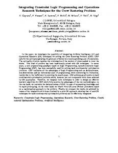
function ACsolver Input Π: r-ground program; B: set of ground regular literals; Output hA, truei where A is a regular part of an answer set of Π containing B; false if there is no such answer set; begin S := Cn(ΠR ∪ ΠM , B); if S is inconsistent return false; if β(ΠD , S) is a constraint program then O := c solve(β(ΠD , S), query(Π, S)); if O = false then return(false) if O = hC, truei and p ∈ S or not p ∈ S for any regular atom p then return(hS, truei); pick a regular literal l such that l, (not l) ∈ / S; O := ACsolver (Π, S ∪ {l}) ; if O = false return ACsolver (Π, S ∪ {not l}); else return O; end Figure 1: The ACsolver algorithm

Finally, by β(Π, B) where B is a set of regular ground literals, we will denote the program obtained from Π by (a) removing the rules whose body is falsified by B, and (b) removing literals of B from the remaining rules of the program. Function ACsolver Now we are ready to present the main function (see Figure 1), ACsolver , which takes an r-ground AC(C) program Π and a set B of ground regular literals as inputs and returns an answer set of Π containing B. If no such answer set exists the program returns false. Of course the actual output will be smaller. Normally we are only interested in the regular parts of Π’s answer sets. The algorithm can be easily expended to return a solution of the set C of constraints returned by c solve. If required, this information can be used to output relevant mixed and defined literals. Let us trace this algorithm for ACsolver (gr(P ), ∅). We already computed the value, S0 of Cn(gr(PR ∪ PM ), ∅). S0 is consistent, β(gr(P )D , S0 ) = gr(P )D and, as has been shown above, query(gr(P ), S0 ) returns Q0 = acceptable time(T0 ). Function c solve(gr(PD ), Q0 ) returns true together with a collection of constraints, say, C0 = 10 ≤ T0 ∧ T0 ≤ 20. For every t0 satisfying C0 , atom acceptable time(t0 ) belongs to an answer set of gr(P ) compatible with S0 . The only regular atom undecided by S0 is ¬occurs(a, 1). Suppose that ACsolver selects this atom and calls ACsolver (P, S1 ) where S1 = S0 ∪ {¬occurs(a, 1)}. Using rule (12) of gr(P ), function Cn(gr(PR ∪ PM ), S1 ) returns S2 = S1 ∪ {not occurs(a, 1)}. Function query(gr(P ), S2 ) returns

Q1 = acceptable time(T0 ) ∧ not acceptable time(T1 ). The possible answer returned by c solve(gr(PD ), Q1 ) may be, say, C1 = 10 ≤ T0 ≤ 20 ∧ T1 < 10 ∧ 20 < T1 < 100 ∧ 120 < T1 . Finally, ACsolver (gr(P ), ∅) returns S2 . (Of course the slightly modified solver can also return C1 , or even some of its solutions). If ACsolver were to select not ¬occurs(a, 1) instead of ¬occurs(a, 1), then the returned value would be S3 = S0 ∪ {not ¬occurs(a, 1), not occurs(a, 1)}. The algorithm is only correct for programs satisfying a number of safety conditions. In particular the usual safety conditions required for correctness of ASP and constraint solvers should be expanded by the following requirement: every middle rule of a program contains a mixed literal, and every constraint variable occurring in a middle rule of the program should occur in a mixed predicate from this rule. The following example shows why the condition is necessary. Consider a program #csort(s). #def ined d(s), e(s). s(0..2). p ← e(Y ). d(1). d(2). e(Y ) ← d(Y ), Y < 2. Every answer set of this program contains d(1), d(2), and p. Our algorithm however may also return sets not containing p. This happens when the algorithm picks literal not p, and c solve returns, say, Y = 0.

4

Representing Knowledge in AC(C)

Several examples presented in this section are meant to illustrate the use of AC(C) for knowledge representation. None of the examples can successfully run with traditional ASP solvers while all of them are easily solvable by the AC(C) solvers. We start with a simple planning and scheduling example: Example 2 [Planning and Scheduling] John, who is currently at work, needs to be in his doctor’s office in one hour carrying the insurance card and money to pay for the visit. The card is at home and money can be obtained from the nearby ATM. John knows the minimum time (in minutes) needed to travel between the relevant locations. Can he find a plan to make it on time? (assuming of course that there will be no delays and the actual time of travel will be the minimum time). To solve the problem we will divide it into two parts: planning and scheduling. The former can be solved by standard ASP based methods. We use variables P for people, L for locations, O for objects (cash and the insurance card), and S for steps of the planned trajectory. We will need an action go to(P, L) and fluents at loc(P, L), at loc(O, L), and has(P, O) with selfexplanatory intuitive meaning. (To simplify the solution we assume that person P automatically gets the

object O when both, P and O, share the same location). The transition diagram whose states are collections of fluents describing possible physical states of the domain and arcs are labeled by actions is defined by causal laws written as logic programming rules. For instance, direct effects of the actions are described by the rule holds(at loc(P,L),S1) ← next(S1, S0), occurs(go to(P,L),S0). Indirect effects will be captured by the corresponding relationships between fluents: holds(has(P,O),S) ← holds(at loc(P,L),S), holds(at loc(P,O),S). holds(at loc(O,L),S) ← holds(at loc(P,L),S), holds(has(P,O),S). ¬holds(at loc(X,L2),S) ← holds(at loc(X,L1),S), L1 6= L2. The problem of representing the unchanged fluents is solved by the inertia axioms (variable F is used for fluents): holds(F,S1) ← next(S1,S0), holds(F,S0), not ¬holds(F,S1). ¬holds(F,S1) ← next(S1,S0), ¬holds(F,S0),not holds(F,S1). John’s goal and his options will be described by the rules: occurs(go to(john,L),S) or ¬occurs(go to(john,L),S). goal(S) ← holds(at loc(john,doctor),S), holds(has(john,card),S), holds(has(john,cash),S). succeed ← goal(S). ← not succeed. Let us denote the above program with initial conditions and sort step defined as a collection of integers from 0 to n by Drn . Normally ASP planning is performed by computing answer sets of Drn for n = 1, 2, . . .. The desired plans can be easily extracted from the answer sets of the first consistent program Drk . A possible plan returned by this planning method can be, say, [go to(john,home), go to(john,atm),go to(john,doctor)]. Now we concentrate on the scheduling part of the problem. Actual time will range from 0 to 1440 (number of minutes in 24 hours). The schedule should assign time T to each step S of the plan. This will be achieved by introducing a mixed relation at(S, T ) and specifying the necessary constraints, e.g.,

← next(S1, S0), at(S0, T 0), at(S1, T 1), T 1 < T 0. ← goal(S), at(0, T 1), at(S, T 2), T 2 − T 1 > 60. ← next(S1, S0), occurs(go to(john, home), S0), holds(at loc(john, of f ice), S0), at(S0, T 0), at(S1, T 1), T 0 − T 1 > −20. The first rule requires time to be a monotonic function of steps; the second guarantees that the trip does not take more than an hour; the third assumes that the trip from office to home takes at least twenty minutes. Other constraints are added in a similar fashion. Let us denote the resulting program by Dn . Given this program the ACsolver will return an answer set of Dn , containing a plan, say [occurs(go to(john,home),0), occurs(go to(john,atm),1), occurs(go to(john,doctor),2)] and a schedule, say, at(0, 0), at(1, 20), at(2, 35), at(3, 55) for executing its actions. It is guaranteed that if John performs the corresponding actions as scheduled he will get to see his doctor on time. If there is no plan of length n satisfying the desired conditions the program Dn has no answer sets. The primitive constraints which occur in the middle rules of Dn are so called difference constraint. We have an implementation of ACsolver which works for the language AC(C) parametrized by such constraints. The current implementation, Suryad , has other limitations - it does not allow defined predicates and regular predicates in the heads of middle rules. Of course Dn satisfies this condition and Suryad returns the answers almost instantaneously. In our next example we illustrate the use of AC(C) extended by consistency restoring rules of CR-Prolog. Example 3 [Planning with Weak Constraints] Let us now consider a variant of the story from Example 2 in which the requirement “the trip does not take more than an hour ” is replaced “the trip does not take more than an hour, but John prefers to make it in 50 minutes”. The new information can be encoded by the defeasible rule which says that under normal circumstances the trip will be made in 50 minutes (or less). ← goal(S), at(0, T 1), at(S, T 2), T 2 − T 1 > 50, not ab(S).

The CR-rule

the safety condition of ACsolver. The problem can be remedied by:

ab(S) ← + step(S). allows, when necessary, consider exceptions to this rule. If John can get to the doctor’s office in 50 minutes the program will find the corresponding plan and a proper schedule for its actions. If time constraints of the problem require time from interval (50, 60] the CR-rule will be used to defeat the weak constraint above and find a possible plan, say, requiring 55 minutes. The desired solutions can be easily found by Suryad . Example 4 [Using Defined Predicates] Let us now consider an extension of the John’s problem from Example 2 by assuming that John always travels in a cab and that the cab rate is $2.45 per minute. John knows the amount of money in his bank account as well as the amount he needs to pay to the doctor. Now he needs not only get to the doctor on time and ready but also make sure that he has enough money for the visit. To solve the problem one may try to encode this knowledge by the following rules: bank account(john, 200). doctor payment(130). taxi rate(2.45). enough money(P) ← goal(S), at(0,T1), at(S,T2), money needed(P,T1,T2,Y1), bank account(P,Y2), Y2 - Y1 ≥ 0. money needed(P,T1,T2,Y) ← doctor payment(Y1), cab payment(T1,T2,Y2), Y = Y1 + Y2. cab payment(T1,T2,Y) ← taxi rate(Rate), Y = Rate * (T2 - T1).

(a) Introducing a new defined relation d specified by the rule d(P,T1,T2,Y1,Y2) ← money needed(P,T1,T2,Y1), bank account(P,Y2), Y2 - Y1 ≥ 0. (b) Introducing a new mixed relation md (P, Y 1, Y 2) whose parameters are obtained from parameters of d by dropping those constraint parameters which occur in the mixed predicates of the middle rule of enough money. (c) Replacing the definition of enough money by the new rule enough money(P) ← goal(S), at(0,T1), at(S,T2), m d(P,Y1,Y2). d(P,T1,T2,Y1,Y2). It is not difficult to show that the transformed program is equivalent to the original one modulo the new predicates. The safety condition now is satisfied and ACsolver can be used to find the answer. The new program has defined predicates, regular predicates in the heads of middle rules and linear constraints and thus can not be run on Suryad . However, we have a second prototype implementation, ACengine, whose (c solve) algorithm is implemented via constraint logic programming system CLP(R) (Jaffar et al. 1992) with constructive negation (Stuckey 1991) which is suitable for solving this problem. The only change necessary to satisfy syntactic restrictions of ACengine consists in replacing disjunction p or ¬p by two rules p ← not ¬p and ¬p ← not p.

5 Since at the final state of the trajectory John should have enough money to pay the doctor and the taxi driver, we expand this program by a rule ← enough money(john). It is natural to declare enough money as a regular predicate, and the rest, except the mixed predicate at and the primitive constraints, are defined predicates. It is not difficult to check that the resulting program, E, has an answer set and that any answer set of this program will contain enough money(john). Notice however that ACsolver will not be able to compute answer sets of E because the definition of enough money(P ) violates

Conclusion

In this paper we introduced a knowledge representation language AC(C) extending the syntax and semantics of ASP and CR-Prolog, gave some examples of its use for knowledge representation, and presented an algorithm, ACsolver, for computing answer sets of AC(C) programs. The algorithm does not require full grounding of a program and combines “classical” ASP solving methods with constraint logic programming techniques and CR-Prolog based abduction. The AC(C) based approach often allows to solve problems which are impossible to solve by more traditional ASP solving techniques. We believe that further investigation of the language and development of more efficient and reliable solvers for its programs can help to substantially

expand the domain of applicability of the answer set programming paradigm. The work is based on previous results by S. Baselice, P. Bonatti, and the authors. In (Elkabani, Pontelli, & Son 2005), an algorithm is developed to combine ASP computation with constraint solving for the purpose of reasoning with ASP aggregates. Their language however does not allow classification of predicates and hence does not avoid grounding of variables (except the variables which are local w.r.t. the aggregates). Interesting line of work investigates ways of replacing ASP programs by the corresponding constraint programs (see for instance (Dovier, Formisano, & Pontelli 2007)). We hope that our approach will prove more attractive from the standpoint of knowledge representation and also more efficient but this is of course a matter for further research. There is also a substantial amount of work on the development of a generalization of ASP by rules which allows arbitrary “constraints atoms” (Marek & Truszczynski 2004; Liu et al. 2007). It remains to be seen if work on the development of AC(C) solvers can profit from insights from this work.

6

Acknowledgments

This work was supported in part by NASA contract NASA-NEG05GP48G and ATEE/DTO contract ASU06-C-0143.

References Apt, K., and Bezem, M. 1991. Acyclic programs. New Generation Computing 9(3,4):335–365. Babovich, Y., and Maratea, M. 2004. Cmodels-2: SAT-based answer set solver enhanced to non-tight programs. In International Conference on Logic Programming and Nonmonotonic Reasoning, LPNMR-05. Balduccini, M., and Gelfond, M. 2003. Logic Programs with Consistency-Restoring Rules. In Doherty, P.; McCarthy, J.; and Williams, M.-A., eds., International Symposium on Logical Formalization of Commonsense Reasoning, AAAI 2003 Spring Symposium Series, 9–18. Balduccini, M.; Gelfond, M.; and Nogueira, M. 2006. Answer set based design of knowledge systems. Annals of Mathematics and Artificial Intelligence 47:183–219. Balduccini, M. 2004. USA-Smart: Improving the Quality of Plans in Answer Set Planning. In PADL’04, Lecture Notes in Artificial Intelligence (LNCS). Balduccini, M. 2007. CR-MODELS: An inference engine for CR-Prolog. In Baral, C.; Brewka, G.; and Schlipf, J., eds., Proceedings of the 9th International Conference on Logic Programming and Non-Monotonic Reasoning (LPNMR’07), volume 3662 of Lecture Notes in Artificial Intelligence, 18–30. Springer. Baral, C.; Chancellor, K.; Tran, N.; Tran, N.; Joy, A.; and Berens, M. 2004. A knowledge based approach for representing and reasoning about cell signalling

networks. In Proceedings of European Conference on Computational Biology, Supplement on Bioinformatics, 15–22. Baral, C. 2003. Knowledge Representation, Reasoning, and Declarative Problem Solving. Cambridge University Press. Baselice, S.; Bonatti, P. A.; and Gelfond, M. 2005. Towards an integration of answer set and constraint solving. In Proceedings of ICLP-05, 52–66. Brooks, D. R.; Erdem, E.; Minett, J. W.; and Ringe, D. 2005. Character-based cladistics and answer set programming. In Proceedings of International Symposium on Practical Aspects of Declarative Languages, 37–51. Chen, W.; Swift, T.; and Warren, D. S. 1995. Efficient top-down computation of queries under the wellfounded semantics. Journal of Logic Programming 24(3):161–201. Clark, K. 1978. Negation as failure. In Gallaire, H., and Minker, J., eds., Logic and Data Bases. Plenum Press. 293–322. Dovier, A.; Formisano, A.; and Pontelli, E. 2007. An experimental comparison of constraint logic programming and answer set programming. In Proceedings of AAAI07, 1622–1625. Eiter, T.; Leone, N.; Mateis, C.; Pfeifer, G.; and Scarcello, F. 1997. A deductive system for nonmonotonic reasoning. In International Conference on Logic Programming and Nonmonotonic Reasoning, LPNMR97, LNAI 1265, 363–374. Springer Verlag, Berlin. Elkabani, I.; Pontelli, E.; and Son, T. C. 2005. Smodelsa - a system for computing answer sets of logic programs with aggregates. In LPNMR, 427–431. Gebser, M.; Kaufman, B.; Neumann, A.; and Schaub, T. 2007. Conflict-driven answer set enumeration. In Baral, C.; Brewka, G.; and Schlipf, J., eds., Proceedings of the 9th International Conference on Logic Programming and Nonmonotonic Reasoning (LPNMR’07), volume 3662 of lnai, 136–148. Springer. Gelfond, M., and Lifschitz, V. 1991. Classical negation in logic programs and disjunctive databases. New Generation Computing 9(3/4):365–386. Giunchiglia, E.; Lierler, Y.; and Maratea, M. 2006. Answer set programming based on propositional satisfiability. Journal of Automated Reasoning 36:345–377. Jaffar, J., and Maher, M. J. 1994. Constraint Logic Programming. Journal of Logic Programming 19/20:503–581. Jaffar, J.; Michaylov, S.; Stuckey, P. J.; and Yap, R. H. C. 1992. The CLP(R) language and system. ACM Transactions on Programming Languages and Systems 14(3):339–395. Leone, N.; Pfeifer, G.; Faber, W.; Eiter, T.; Gottlob, G.; Perri, S.; and Scarcello, F. 2006. The DLV system for knowledge representation and reasoning. ACM Transactions on Computational Logic 7:499–562.

Lin, F., and Zhao, Y. 2004. ASSAT: Computing answer sets of a logic program by SAT solvers. Artificial Intelligence 157(1-2):115–137. Liu, L.; Pontelli, E.; Son, T. C.; and Truszczynski, M. 2007. Logic programs with abstract constraint atoms: The role of computations. In Proceedings of ICLP-07, 286–301. Marek, V. W., and Truszczynski, M. 1993. Nonmonotonic logics; context dependent reasoning. Springer Verlag, Berlin. Marek, V. W., and Truszczynski, M. 1999. Stable models and an alternative logic programming paradigm. The Logic Programming Paradigm: a 25-Year Perspective. Springer Verlag, Berlin. 375–398. Marek, V. W., and Truszczynski, M. 2004. Logic programs with abstract constraint atoms. In Proceedings of AAAI04, 86–91. Marriott, K., and Stuckey, P. J. 1998. Programming with Constraints: an Introduction. Cambridge, MA: MIT Press. Mellarkod, V. S., and Gelfond, M. 2007. Enhancing asp systems for planning with temporal constraints. In LPNMR 2007, 309–314. Niemela, I., and Simons, P. 1997. Smodels - an implementation of the stable model and well-founded semantics for normal logic programs. In Proceedings of the 4th International Conference on Logic Programming and Non-Monotonic Reasoning (LPNMR’97), volume 1265 of Lecture Notes in Artificial Intelligence (LNCS), 420–429. Niemela, I.; Simons, P.; and Soininen, T. 2002. Extending and implementing the stable model semantics. Artificial Intelligence 138(1–2):181–234. Niemela, I. 1999. Logic programs with stable model semantics as a constraint programming paradigm. Annals of Mathematics and Artificial Intelligence 25(3– 4):241–27. SICStus Prolog. 2007. SICStus Prolog User’s Manual Version 4. http://www.sics.se/isl/sicstuswww/site/index.html. Soininen, T., and Niemella, I. 1998. Developing a declarative rule language for applications in product configuration. In Proceedings of International Symposium on Practical Aspects of Declarative Languages, 305–319. Stuckey, P. J. 1991. Constructive negation for constraint logic programming. In LICS, 328–339. Van Hentenryck, P. 1989. Constraint Satisfaction in Logic Programming. Cambridge, MA: MIT Press.