Integrating Boolean and Mathematical Solving: Foundations, Basic Algorithms and Requirements ? Gilles Audemard12 , Piergiorgio Bertoli1 , Alessandro Cimatti1 , Artur Kornilowicz13 , and Roberto Sebastiani14 1
3
ITC-IRST, Povo, Trento, Italy {audemard,bertoli,cimatti,kornilow}@itc.it 2 LSIS, University of Provence, Marseille, France Institute of Computer Science, University of Bialystok, Poland 4 DIT, Universit` a di Trento, Povo, Trento, Italy
[email protected]
Abstract. In the last years we have witnessed an impressive advance in the efficiency of boolean solving techniques, which has brought large previously intractable problems at the reach of state-of-the-art solvers. Unfortunately, simple boolean expressions are not expressive enough for representing many real-world problems, which require handling also integer or real values and operators. On the other hand, mathematical solvers, like computer-algebra systems or constraint solvers, cannot handle efficiently problems involving heavy boolean search, or do not handle them at all. In this paper we present the foundations and the basic algorithms for a new class of procedures for solving boolean combinations of mathematical propositions, which combine boolean and mathematical solvers, and we highlight the main requirements that boolean and mathematical solvers must fulfill in order to achieve the maximum benefits from their integration. Finally we show how existing systems are captured by our framework.
1
Motivation and goals
In the last years we have witnessed an impressive advance in the efficiency of boolean solving techniques (SAT), which has brought large previously intractable problems at the reach of state-of-the-art solvers. 1 As a consequence, some hard real-world problems have been successfully solved by encoding them into SAT. Propositional planning [KMS96] and boolean model-checking [BCCZ99] are among the best achievements. ?
1
This work is sponsored by the CALCULEMUS! IHP-RTN EC project, contract code HPRN-CT-2000-00102, and has thus benefited of the financial contribution of the Commission through the IHP programme. SAT procedures are commonly called solvers in the SAT community, although the distinction between solving, proving and computing services may suggest to call them provers.
Unfortunately, simple boolean expressions are not expressive enough for representing many real-world problems. For example, problem domains like temporal reasoning, resource planning, verification of systems with numerical data or of timed systems, require handling also constraints on integer or real quantities (see, e.g., [ACG99,WW99,CABN97,MLAH01]). Moreover, some problem domains like model checking often require an explicit representation of integers and arithmetic operators, which cannot be represented efficiently by simple boolean expressions (see, e.g., [CABN97,MLAH01]). On the other hand, mathematical solvers, like computer-algebra systems or constraint solvers, cannot handle efficiently problems involving heavy boolean search, or do not handle them at all. In 1996 we have proposed a new general approach to build domain-specific decision procedures on top of SAT solvers [GS96,GS00]. The basic idea was to decompose the search into two orthogonal components, one purely propositional component and one “boolean-free” domain-specific component and to use a (modified) Davis Putnam Longemann Loveland (DPLL) SAT solver [DLL62] for the former and a pure domain-specific procedure for the latter. So far the SAT based approach proved very effective in various problem domains like, e.g., modal and description logics [GS00], temporal reasoning [ACG99], resource planning [WW99]. In this paper we present the foundations and the basic algorithms for a new class of procedures for solving boolean combinations of mathematical propositions, which integrate SAT and mathematical solvers, and we highlight the main requirement SAT and mathematical solvers must fulfill in order to achieve the maximum benefits from their integration. The ultimate goal is to develop solvers able to handle complex problems like those hinted above. The paper is structured as follows. In Section 2 we describe formally the problem we are addressing. In Section 3 we present the logic framework on which the procedures are based. In Section 4 we present a generalized search procedure which combine boolean and mathematical solvers and introduce some efficiency issues. In Section 5 we highlight the main requirements that boolean and mathematical solvers must fulfill in order to achieve the maximum benefits from their integration. In Section 6 we briefly describe some existing systems which are captured by our framework,and our own implemented procedure. For lack of space, in this paper we omit the proofs of all the theoretical results presented, which can be found in [Seb01].
2
The problem
We address the problem of checking the satisfiability of boolean combinations of primitive and mathematical propositions. Let D be the domain of either integer numbers Z or real numbers R, with the respective set OPD of arithmetical operators {+, −, ·, /, mod} or {+, −, ·, /} respectively. Let {⊥, >} denote the f alse and true boolean values. Given the standard boolean connectives {¬, ∧} and math operators {=, 6=, >, , < , ≥, ≤}; – if ϕ1 is a Math-formula, then ¬ϕ1 is a Math-formula; – if ϕ1 , ϕ2 are Math-formulas, then (ϕ1 ∧ ϕ2 ) is a Math-formula. For instance, A1 ∧ ((v1 + 5.0) ≤ (2.0 · v3 )) and A2 ∧ ¬(((2 · v1 ) mod v2 ) > 5) are Math-formulas. 2 Notationally, we use the lower case letters t, t1 , ... to denote Math-terms, and the Greek letters α, β, ϕ, ψ to denote Math-formulas. We use the standard abbreviations, that is: “ϕ1 ∨ ϕ2 ” for “¬(¬ϕ1 ∧ ¬ϕ2 )”, “ϕ1 → ϕ2 ” for “¬(ϕ1 ∧ ¬ϕ2 )”, “ϕ1 ↔ ϕ2 ” for “¬(ϕ1 ∧¬ϕ2 )∧¬(ϕ2 ∧¬ϕ1 )”, “>” for any valid formula, and “⊥” for “¬>”. When this does not cause ambiguities, we use the associativity and precedence rules of arithmetical operators to simplify the appearance of Math-terms; e.g, we write “(c1 (v2 − v1 ) − c1 v3 + c3 v4 )” instead of “(((c1 · (v2 − v1 )) − (c1 · v3 )) + (c3 · v4 ))”. We call interpretation a map I which assigns D values and boolean values to Math-terms and Math-formulas respectively and preserves constants and arithmetical operators:3 – – – – 2
3
I(Ai ) ∈ {>, ⊥}, for every Ai ∈ A; I(ci ) = ci , for every ci ∈ C; I(vi ) ∈ D, for every vi ∈ V; I(t1 ⊗ t2 ) = (I(t1 ) ⊗ I D (t2 )), for all Math-terms t1 , t2 and ⊗ ∈ OP D .
The assumption that the domain is the whole Z or R is not restrictive, as we can restrict the domain of any variable vi at will by adding to the formula some constraints like, e.g., (v1 6= 0.0), (v1 ≤ 5.0), etc. Here we make a little abuse of notation with the constants and the operators in OP D . In fact, e.g., we denote by the same symbol “+” both the language symbol in I D (t1 + t2 ) and the arithmetic operator in (I D (t1 ) + I D (t2 )). The same discourse holds for the constants ci ∈ C and also for the operators {=, 6=, >, ; |= (t1 ./ t2 ), ./ ∈ {=, 6=, >, , I(v1 ) = 1.1, and I(v2 ) = 0.6. For every ϕ1 and ϕ2 , we say that ϕ1 |= ϕ2 if and only if I |= ϕ2 for every I such that I |= ϕ1 . We also say that |= ϕ (ϕ is valid ) if and only if I |= ϕ for every I. It is easy to verify that ϕ1 |= ϕ2 if and only if |= ϕ1 → ϕ2 , and that |= ϕ if and only if ¬ϕ is unsatisfiable.
3 3.1
The formal framework Basic definitions and results
Definition 1. We call atom any Math-formula that cannot be decomposed propositionally, that is, any Math-formula whose main connective is not a boolean operator. A literal is either an atom (a positive literal) or its negation (a negative literal). Examples of literals are, A1 , ¬A2 , (v1 + 5.0 ≤ 2.0v3 ), ¬((2v1 mod v2 ) > 5). If l is a negative literal ¬ψ, then by “¬l” we conventionally mean ψ rather than ¬¬ψ. We denote by Atoms(ϕ) the set of atoms in ϕ. Definition 2. We call a total truth assignment µ for a Math-formula ϕ a set µ = {α1 , . . . , αN , ¬β1 , . . . , ¬βM , A1 , . . . , AR , ¬AR+1 , . . . , ¬AS }, (1) such that every atom in Atoms(ϕ) occurs as either a positive or a negative literal in µ. A partial truth assignment µ for ϕ is a subset of a total truth assignment for ϕ. If µ2 ⊆ µ1 , then we say that µ1 extends µ2 and that µ2 subsumes µ1 . A total truth assignment µ like (1) is interpreted as a truth value assignment to all the atoms of ϕ: αi ∈ µ means that αi is assigned to >, ¬βi ∈ µ means that βi is assigned to ⊥. Syntactically identical instances of the same atom are always assigned identical truth values; syntactically different atoms, e.g., (t1 ≥ t2 ) and (t2 ≤ t1 ), are treated differently and may thus be assigned different truth values. Notationally, we use the Greek letters µ, η to represent truth assignments. We often write a truth assignment µ as the conjunction of its elements. To this extent, we say that µ is satisfiable if the conjunction of its elements is satisfiable.
Definition 3. We say that a total truth assignment µ for ϕ propositionally satisfies ϕ, written µ |=p ϕ, if and only if it makes ϕ evaluate to >, that is, for all sub-formulas ϕ1 , ϕ2 of ϕ: µ |=p ϕ1 , ϕ1 ∈ Atoms(ϕ) ⇐⇒ ϕ1 ∈ µ; µ |=p ¬ϕ1 ⇐⇒ µ 6|=p ϕ1 ; µ |=p ϕ1 ∧ ϕ2 ⇐⇒ µ |=p ϕ1 and µ |=p ϕ2 . We say that a partial truth assignment µ propositionally satisfies ϕ if and only if all the total truth assignments for ϕ which extend µ propositionally satisfy ϕ. From now on, if not specified, when dealing with propositional satisfiability we do not distinguish between total and partial assignments. We say that ϕ is propositionally satisfiable if and only if there exist an assignment µ such that µ |=p ϕ. Intuitively, if we consider a Math-formula ϕ as a propositional formula in its atoms, then |=p is the standard satisfiability in propositional logic. Thus, for every ϕ1 and ϕ2 , we say that ϕ1 |=p ϕ2 if and only if µ |=p ϕ2 for every µ such that µ |=p ϕ1 . We also say that |=p ϕ (ϕ is propositionally valid ) if and only if µ |=p ϕ for every assignment µ for ϕ. It is easy to verify that ϕ1 |=p ϕ2 if and only if |=p ϕ1 → ϕ2 , and that |=p ϕ if and only if ¬ϕ is propositionally unsatisfiable. Notice that |=p is stronger than |=, that is, if ϕ1 |=p ϕ2 , then ϕ1 |= ϕ2 , but not vice versa. E.g., (v1 ≤ v2 ) ∧ (v2 ≤ v3 ) |= (v1 ≤ v3 ), but (v1 ≤ v2 ) ∧ (v2 ≤ v3 ) 6|=p (v1 ≤ v3 ). Example 1. Consider the following math-formula ϕ: ϕ = {¬(2v2 − v3 > 2) ∨ A1 } ∧ {¬A2 ∨ (2v1 − 4v5 > 3)} ∧ {(3v1 − 2v2 ≤ 3) ∨ A2 } ∧ {¬(2v3 + v4 ≥ 5) ∨ ¬(3v1 − v3 ≤ 6) ∨ ¬A1 } ∧ {A1 ∨ (3v1 − 2v2 ≤ 3)} ∧ {(v1 − v5 ≤ 1) ∨ (v5 = 5 − 3v4 ) ∨ ¬A1 } ∧ {A1 ∨ (v3 = 3v5 + 4) ∨ A2 }. The truth assignment given by the underlined literals above is: µ = {¬(2v2 −v3 > 2), ¬A2 , (3v1 −2v2 ≤ 3), (v1 −v5 ≤ 1), ¬(3v1 −v3 ≤ 6), (v3 = 3v5 +4)}. Notice that the two occurrences of (3v1 − 2v2 ≤ 3) in rows 3 and 5 of ϕ are both assigned >. µ is an assignment which propositionally satisfies ϕ, as it sets to true one literal of every disjunction in ϕ. Notice that µ is not satisfiable, as both the following sub-assignments of µ {(3v1 − 2v2 ≤ 3), ¬(2v2 − v3 > 2), ¬(3v1 − v3 ≤ 6)} {(v1 − v5 ≤ 1), (v3 = 3v5 + 4), ¬(3v1 − v3 ≤ 6)} do not have any satisfying interpretation.
(2) (3) 3
Definition 4. We say that a collection M = {µ1 , . . . , µn } of (possibly partial) assignments propositionally satisfying ϕ is complete if and only if _ |=p ϕ ↔ µj . (4) j
where each assignment µj is written as a conjunction of its elements. M is complete in the sense that, for every total assignment η such that η |=p ϕ, there exists µj ∈ M such that µj ⊆ η. Therefore M is a compact representation of the whole set of total assignments propositionally satisfying ϕ. Notice however that ||M|| is worst-case exponential in the size of ϕ, though typically much smaller than the set of all total assignments satisfying ϕ. Definition 5. We say that a complete collection M = {µ1 , . . . , µn } of assignments propositionally satisfying ϕ is non-redundant if for every µj ∈ M, M \ {µj } is no more complete, it is redundant otherwise. M is strongly non-redundant if, for every µi , µj ∈ M, (µ1 ∧ µ2 ) is propositionally unsatisfiable. It is easy to verify that, if M is redundant, then µi ⊆ µj for some i, j, and that, if M is strongly non-redundant, then it is non-redundant too, but the vice versa does not hold. Example 2. Let ϕ := (α ∨ β ∨ γ) ∧ (α ∨ β ∨ ¬γ), α, β and γ being atoms. Then 1. {{α, β, γ}, {α, β, ¬γ}, {α, ¬β, γ}, {α, ¬β, ¬γ}, {¬α, β, γ}, {¬α, β, ¬γ}} is the set of all total assignments propositionally satisfying ϕ; 2. {{α}, {α, β}, {α, ¬γ}, {α, β}, {β}, {β, ¬γ}, {α, γ}, {β, γ}} is complete but redundant; 3. {{α}, {β}} is complete, non redundant but not strongly non-redundant; 4. {{α}, {¬α, β}} is complete and strongly non-redundant. 3 Theorem 1. Let ϕ be a Math-formula and let M = {µ1 , . . . , µn } be a complete collection of truth assignments propositionally satisfying ϕ. Then ϕ is satisfiable if and only if µj is satisfiable for some µj ∈ M. 3.2
Decidability and complexity
Having a Math-formula ϕ, it is always possible to find a complete collection of satisfying assignments for ϕ (see later). Thus from Theorem 1 we have trivially the following fact. Proposition 1. The satisfiability problem for a Math-formula over atoms of a given class is decidable if and only if the satisfiability of sets of literals of the same class is decidable.
For instance, the satisfiability of a set of linear constraints on R or on Z, or a set of non-linear constraints on R is decidable, whilst a set of non-linear (polynomial) constraints on Z is not decidable (see, e.g., [RV01]). Consequently, the satisfiability of Math-formulas over linear constraints on R or on Z, or over nonlinear constraints on R is decidable, whilst the satisfiability of Math-formulas over non-linear constraints over Z is undecidable. For the decidable cases, as standard boolean formulas are a strict subcase of Math-formulas, it follows trivially that deciding the satisfiability of Mathformulas is “at least as hard” as boolean satisfiability. Proposition 2. The problem of deciding the satisfiability of a Math-formula ϕ is NP-hard. Thus, deciding satisfiability is computationally very expensive. The complexity upper bound may depend on the kind of mathematical problems we are dealing. For instance, if we are dealing with arithmetical expressions over bounded integers, then for every I we can verify I |= ϕ in a polynomial amount of time, and thus the problem is also NP-complete.
4
A generalized search procedure
Theorem 1 allows us to split the notion of satisfiability of a Math-formula ϕ into two orthogonal components: – a purely boolean component, consisting of the existence of a propositional model for ϕ; – a purely mathematical component, consisting of the existence of an interpretation for a set of atomic (possibly negated) mathematical propositions. These two aspects are handled, respectively, by a truth assignment enumerator and by a mathematical solver. Definition 6. We call a truth assignment enumerator a total function Assign Enumerator which takes as input a Math-formula ϕ and returns a complete collection {µ1 , . . . , µn } of assignments satisfying ϕ. Notice the difference between a truth assignment enumerator and a standard boolean solver: a boolean solver has to find only one satisfying assignment —or to decide there is none— while an enumerator has to find a complete collection of satisfying assignments. (We will show later how some boolean solvers can be modified to be used as enumerators.) We say that Assign Enumerator is – strongly non-redundant if Assign Enumerator(ϕ) is strongly non-redundant, for every ϕ, – non-redundant if Assign Enumerator(ϕ) is non-redundant for every ϕ, – redundant otherwise.
boolean Math-SAT(f ormula ϕ, assignment & µ, interpretation & I) do µ := N ext(Assign Enumerator(ϕ)) /* next in {µ1 , ..., µn } */ if (µ 6= N ull) I :=MathSolver(µ); while ((I = N ull) and (µ 6= N ull)) if (I = 6 N ull) then return True; /* a D-satisfiable assignment found */ else return False; /* no D-satisfiable assignment found */
Fig. 1. Schema of the generalized search procedure for D-satisfiability.
Definition 7. We call a mathematical solver a total function MathSolver which takes as input a set of (possibly negated) atomic Math-formulas µ and returns an interpretation satisfying µ, or N ull if there is none. The general schema of a search procedure for satisfiability is reported in Figure 1. Math-SAT takes as input a formula ϕ and (by reference) an initially empty assignment µ and an initially null interpretation I. For every assignment µ in the collection {µ1 , .., µn } generated by Assign Enumerator(ϕ), Math-SAT invokes MathSolver over µ, which either returns a interpretation satisfying µ, or N ull if there is none. This is done until either one satisfiable assignment is found, or no more assignments are available in {µ1 , ..., µn }. In the former case ϕ is satisfiable, in the later case it is not. Math-SAT performs at most ||M|| loops. Thus, if every call to MathSolver terminates, then Math-SAT terminates. Moreover, it follows from Theorem 1 that Math-SAT is correct and complete if MathSolver is correct and complete. Notice that, it is not necessary to check the whole set of total truth assignments satisfying ϕ, rather it is sufficient to check an arbitrary complete collection M of partial assignments propositionally satisfying ϕ, which is typically much smaller. It is very important to notice that the search procedure schema of Figure 1 is completely independent on the kind of mathematical domain we are addressing, once we have a mathematical solver for it. This means that the expressivity of Math-SAT, that is, the kind of math-formulas Math-SAT can handle, depends only on the kind of sets of mathematical atomic propositions MathSolver can handle. 4.1
Suitable Assign Enumerators
The following are the most significant boolean reasoning techniques that we can adapt to be used as assignment enumerators.
Fig. 2. OBDD, Tableau search graph and DPLL search graph for the formula (α ∨ β ∨ γ) ∧ (α ∨ β ∨ ¬γ).
DNF. The simplest technique we can use as an enumerator is the Disjunctive Normal Form (DNF) conversion. A propositional formula ϕ can be converted into a formula DN F (ϕ) by (i) recursively applying DeMorgan’s rewriting rules to ϕ until the result is a disjunction of conjunction of literals, and (ii) removing all duplicated and subsumed disjuncts. The resulting formula is normal, in the sense that DN F (ϕ) is propositionally equivalent to ϕ, and that propositionally equivalent formulas generate the same DNF modulo reordering. By Definition 4, we can see (the set of disjuncts of) DN F (ϕ) as a complete and non-redundant —but not strongly non-redundant— collection of assignments propositionally satisfying ϕ. For instance, in Example 2, the set of assignments at point 2. and 3. are respectively the results of step (i) and (ii) above.
OBDD . A more effective normal form for representing a boolean formula if given by the Ordered Binary Decision Diagrams (OBDDs) [Bry86], which are extensively used in hardware verification and model checking. Given a total ordering v1 , ..., vn on the atoms of ϕ, the OBDD representing ϕ (OBDD(ϕ)) is a directed acyclic graph such that (i) each node is either one of the two terminal nodes T, F , or an internal node labeled by an atom v of ϕ, with two outcoming edges T (v) (“v is true”) and F (v) (“v is false”), (ii) each arc vi → vj is such that vi < vj in the total order. If a node n labeled with v is the root of OBDD(φ) and n1 , n2 are the two son nodes of n through the edges T (v) and F (v) respectively, then n1 , n2 are the roots of OBDD(φ[v = >]) and OBDD(φ[v = ⊥]) respectively. A path from the root of OBDD(ϕ) to T [resp. F ] is a propositional model [resp. counter-model] of ϕ, and the disjunction of such paths is propositionally equivalent to ϕ [resp. ¬ϕ]. Thus, we can see OBDD(ϕ) as a complete collection of assignments propositionally satisfying ϕ. As every pair of paths differ for the truth value of at least one variable, OBDD(ϕ) is also strongly non-redundant. For instance, in Figure 2 (left) the OBDD of the formula in Example 2 is represented. The paths to T are those given by the set of assignments at point 4. of Example 2.
Semantic tableaux. A standard boolean solving technique is that of semantic tableaux [Smu68]. Given an input formula ϕ, in each branch of the search tree the set {ϕ} is decomposed into a set of literals µ by the recursive application of the rules: µ0 ∪ {ϕ1 , ..., ϕn } Vn (∧) µ0 ∪ { i=1 ϕi }
µ0 ∪ {ϕ1 } .... µ0 ∪ {ϕn } W (∨), n µ0 ∪ { i=1 ϕi }
plus analogous rules for (→), (↔), (¬∧), (¬∨), (¬ →), (¬ ↔). The main steps are: – (closed branch) if µ contains both ϕi and ϕi for some subformula ϕi of ϕ, then µ is said to be closed and cannot be decomposed any further; – (solution branch) if µ contains only literals, then it is an assignment such that µ |=p ϕ; – (∧-rule) if µ contains a conjunction, then the latter is unrolled into the set of its conjuncts; – (∨-rule) if µ contains a disjunction, then the search branches on one of the disjuncts. The search tree resulting from the decomposition is such that all its solution branches are assignments in a collection T ableau(ϕ), whose disjunction is propositionally equivalent to ϕ. Thus T ableau(ϕ) is complete, but it may be redundant. For instance, in Figure 2 (center) the search tree of a semantic tableau applied on the formula in Example 2 is represented. The solutions branches give rise to the redundant collection of assignments at point 2. of Example 2. DPLL. The most commonly used boolean solving procedure is DPLL [DLL62]. Given ϕ in input, DPLL tries to build recursively one assignment µ satisfying ϕ, at each step adding a new literal to µ and simplifying ϕ, according to the following steps: – (base) If ϕ = >, then µ propositionally satisfies the original formula, so that µ is returned; – (backtrack) if ϕ = ⊥, µ propositionally falsifies the original formula, so that DPLL backtracks; – (unit propagation) if a literal l occurs in ϕ as a unit clause, then DPLL is invoked recursively on ϕl=> and µ∪{l}, ϕl=> being the result of substituting > for l in ϕ and simplifying; – (split) otherwise, a literal l is selected, and DPLL is invoked recursively on ϕl=> and µ ∪ {l}. If this call succeeds, then the result is returned, otherwise DPLL is invoked recursively on ϕl=⊥ and µ ∪ {¬l}. Standard DPLL can be adapted to work as a boolean enumerator by simply modifying in the base case “µ is returned” with “µ is added to the collection, and backtrack” [GS96,Seb01]. The resulting set of assignments DP LL(ϕ) is complete and strongly nonredundant [Seb01]. For instance, in Figure 2 (right) the search tree of DPLL
applied on the formula in Example 2 is represented. The non closed branches give rise to the set of assignments at point 4. of Example 2. Notice the difference between an OBDD and (the search tree of) DPLL: first, the former is a direct acyclic graph whilst the second is a tree; second, in OBDDs the order of branching variables if fixed a priori, while DPLL can choose each time the best variable to split. 4.2
Non-suitable Assign Enumerators
It is very important to notice that, in general, not every boolean solver can be adapted to work as a boolean enumerator. For instance, many implementations of DPLL include also the following step between unit propagation and split: – (pure literal) if an atom ψ occurs only positively [resp. negatively] in ϕ, then DPLL is invoked recursively on ϕψ=> and µ ∪ {ψ} [resp. ϕψ=⊥ and µ ∪ {¬ψ}]; (we call this variant DPLL+PL). DPLL+PL is complete as a boolean solver, but does not generate a complete collection of assignments, so that it cannot be used as an enumerator. Example 3. If we used DPLL+PL as Assign Enumerator in Math-SAT and gave in input the formula in Example 2, DPLL+PL might return the oneelement collection {{α}}, which is not complete. If α is (x2 + 1 ≤ 0) and β is (y ≤ x), x, y ∈ R, then {α} is not satisfiable, so that Math-SAT would return unsatisfiable. On the other hand, the formula ϕ is satisfiable because, e.g., the assignment {¬α, β} is satisfied by I(x) = 1.0 and I(y) = 0.0.
5
Requirements for Assign Enumerator and MathSolver
Apart from the efficiency of MathSolver —which varies with the kind of problem addressed and with the technique adopted, and will not be discussed here— and that of the SAT solver used —which does not necessarily imply its efficiency as an enumerator— many other factors influence the efficiency of Math-SAT. 5.1
Efficiency requirements for Assign Enumerator
Polynomial vs. exponential space in Assign Enumerator. We would rather Math-SAT require polynomial space. As M can be exponentially big with respect to the size of ϕ, we would rather adopt a generate-check-and-drop paradigm: at each step, generate the next assignment µi ∈ M, check its satisfiability, and then drop it —or drop the part of it which is not common to the next assignment— before passing to the i + 1-step. This means that Assign Enumerator must be able to generate the assignments one at a time. To this extent, both DNF and OBDD are not suitable, as they force generating the whole assignment collection M one-shot. Instead, both semantic tableaux and DPLL are a good choice, as their depth-first search strategy allows for generating and checking one assignment at a time.
Non-redundancy of Assign Enumerator. We want to reduce as much as possible the number of assignments generated and checked. To do this, a key issue is avoiding MathSolver being invoked on an assignment which either is identical to an already-checked one or extends one which has been already found unsatisfiable. This is obtained by using a non-redundant enumerator. To this extent, semantic tableaux are not a good choice. Non-redundant enumerators avoid generating partial assignments whose unsatisfiability is a propositional consequence of those already generated. If M is strongly non-redundant, however, each total assignment η propositionally satisfying ϕ is represented by one and only one µj ∈ M, and every µj ∈ M represents univocally 2|Atoms(ϕ)|−|µj | total assignments. Thus strongly non-redundant enumerators also avoid generating partial assignments covering areas of the search space which are covered by already-generated ones. For enumerators that are not strongly non-redundant, there is a tradeoff between redundancy and polynomial memory. In fact, when adopting a generatecheck-and-drop paradigm, the algorithm has no way to remember if it has already checked a given assignment or not, unless it explicitly keeps track of it, which requires up to exponential memory. Strong non-redundancy instead provides a logical warrant that an already checked assignment will never be checked again.
5.2
Exploiting the interaction between Assign Enumerator and MathSolver
Intermediate assignment checking. If an assignment µ0 is unsatisfiable, then all its extensions are unsatisfiable. Thus, when the unsatisfiability of µ0 is detected during its recursive construction, this prevents checking the satisfiability 0 of all the up to 2|Atoms(ϕ)|−|µ | truth assignments which extend µ0 . Thus, another key issue for efficiency is the possibility of modifying Assign Enumerator so that it can perform intermediate calls to MathSolver and it can take advantage of the (un)satisfiability information returned to prune the search space. With semantic tableaux and DPLL, this can be easily obtained by introducing an intermediate test, immediately before the (∨-rule) and the (split) step respectively, in which MathSolver is invoked on an intermediate assignment µ0 and, if it is inconsistent, the whole branch is cut [GS96,ABC+ 02]. With OBDDs, it is possible to reduce an existing OBDD by traversing it depth-first and redirecting to the F node the paths representing inconsistent assignments [CABN97]. However, this requires generating the non-reduced OBDD anyway.
Generating and handling conflict sets. Given an unsatisfiable assignment µ, we call a conflict set any unsatisfiable sub-assignment µ0 ⊂ µ. (E.g., in Example 1 (2) and (3) are conflict sets for the assignment µ.) A key efficiency issue for Math-SAT is the capability of MathSolver to return the conflict set which has caused the inconsistency of an input assignment, and the capability of Assign Enumerator to use this information to prune search.
For instance, both Belman-Ford algorithm and Simplex LP procedures can produce conflict sets [ABC+ 02,WW99]. Semantic tableaux and DPLL can be enhanced by a technique called mathematical backjumping [HPS98,WW99,ABC+ 02]: when MathSolver(µ) returns a conflict set η, Assign Enumerator can jump back in its search to the deepest branching point in which a literal l ∈ η is assigned a truth value, pruning the search tree below. DPLL can be enhanced also with learning [WW99,ABC+ 02]: the negation of the conflict set ¬η is added in conjunction to the input formula, so that DPLL will never again generate an assignment containing the conflict set η. Generating and handling derived assignments. Another efficiency issue for Math-SAT is the capability of MathSolver to produce an extra assignment η derived deterministically from a satisfiable input assignment µ, and the capability of Assign Enumerator to use this information to narrow the search. For instance, in the procedure presented in [ABC+ 02,ACKS02], MathSolver computes equivalence classes of real variables and performs substitutions which can produce further assignments. E.g., if (v1 = v2 ), (v2 = v3 ) ∈ µ, (v1 − v3 > 2) 6∈ µ and µ is satisfiable, then MathSolver(µ) finds that v1 and v3 belong to the same equivalence class and returns an extra assignment η containing ¬(v1 − v3 > 2), which is unit-propagated away by DPLL. Incrementality of MathSolver. Another efficiency issue of MathSolver is that of being incremental, so that to avoid restarting computation from scratch whenever it is given in input an assignment µ0 such that µ0 ⊃ µ and µ has already proved satisfiable. (This happens, e.g., at the intermediate assignments checking steps.) Thus, MathSolver should “remember” the status of the computation from one call to the other, whilst Assign Enumerator should be able to keep track of the computation status of MathSolver. For instance, it is possible to modify a Simplex LP procedure so that to make it incremental, and to make DPLL call it incrementally after every unit propagation [WW99].
6
Implemented systems
In order to provide evidence of the generality of our approach, in this section we briefly present some examples. First we enumerate some existing procedures which are captured by our framework. Then we present a brief description of our own solver Math-SAT. 6.1
Examples
Our framework captures a significant amount of existing procedure used in various application domains. We briefly recall some of them.
Omega [Pug92] is a procedure used for dependence analysis of software. It is an integer programming algorithm based on an extension of Fourier-Motzkin variable elimination method. It handles boolean combinations of linear constraints by simply pre-computing the DNF of the input formula. TSAT [ACG99] is an optimized procedure for temporal reasoning able to handle sets of disjunctive temporal constraints. It integrates DPLL with a simplex LP tool, adding some form of forward checking and static learning. LPSAT [WW99] is an optimized procedure for Math-formulas over linear real constraints, used to solve problems in the domain of resource planning. It accept only formulas with positive mathematical constraints. LPSAT integrates DPLL with an incremental simplex LP tool, and performs backjumping and learning. SMV+QUAD-CLP [CABN97] integrates OBDDs with a quadratic constraint solver to verify transition systems with integer data values. It performs a form of intermediate assignment checking. DDD [MLAH01] are OBDD-like data structures handling boolean combinations of temporal constraints in the form (x−z ≤ 3), which are used to verify timed systems. They combine OBDDs with an incremental version of Belman-Ford minimal path and cycle detection algorithm. Unfortunately, the last two approaches inherit from OBDDs the drawback of requiring exponential space in worst case. 6.2
A DPLL-based implementation of Math-SAT
In [ABC+ 02,ACKS02] we presented Math-SAT, a decision procedure for Mathformulas over boolean and linear mathematical propositions over the reals. MathSAT uses as Assign Enumerator an implementation of DPLL, and as MathSolver a hierarchical set of mathematical procedures for linear constraints on real variables able to handle theories of increasing expressive power. The latter include a procedure for computing and exploiting equivalence classes from equality constraints like (x = y), a Bellman-Ford minimal path algorithm with cycle detection for handling differences like (x − y ≤ 4), and a Simplex LP procedure for handling the remaining linear constraints. MathSAT implements and uses most of the tricks and optimizations described in Section 5. Technical details can be found in [ABC+ 02]. Math-SAT is available at http://www.dit.unitn.it/~rseba/Mathsat.html. In [ABC+ 02,ACKS02] preliminary experimental evaluations were carried out on tests arising from temporal reasoning [ACG99] and formal verification of timed systems [ACKS02]. In the first class of problems, we have compared our results with the results of the specialized procedure Tsat; although Math-SAT is able to tackle a wider class of problems, it runs faster that the Tsat solver, which is specialized to the problem class. In the second class, we have encoded bounded model checking problems for timed systems into the satisfiability of Math-formulas, and run Math-SAT on them. It turned out that our approach was comparable in efficiency with two well-established model checkers for timed systems, and significantly more expressive [ACKS02].
References [ABC+ 02] G. Audemard, P. Bertoli, A. Cimatti, A. Kornilowicz, and R. Sebastiani. A SAT Based Approach for Solving Formulas over Boolean and Linear Mathematical Propositions. In Proc. CADE’2002., 2002. To appear. Available at http://www.dit.unitn.it/~rseba/publist.html. [ACG99] A. Armando, C. Castellini, and E. Giunchiglia. SAT-based procedures for temporal reasoning. In Proc. European Conference on Planning, CP-99, 1999. [ACKS02] G. Audemard, A. Cimatti, A. Kornilowicz, and R. Sebastiani. SATBased Bounded Model Checking for Timed Systems. 2002. Available at http://www.dit.unitn.it/~rseba/publist.html. [BCCZ99] A. Biere, A. Cimatti, E. Clarke, and Y. Zhu. Symbolic model checking without BDDs. In Proc. CAV’99, 1999. [Bry86] R. E. Bryant. Graph-Based Algorithms for Boolean Function Manipulation. IEEE Transactions on Computers, C-35(8):677–691, August 1986. [CABN97] W. Chan, R. J. Anderson, P. Beame, and D. Notkin. Combining constraint solving and symbolic model checking for a class of systems with non-linear constraints. In Proc. CAV’97, volume 1254 of LNCS, pages 316–327, Haifa, Israel, June 1997. Springer-Verlag. [DLL62] M. Davis, G. Longemann, and D. Loveland. A machine program for theorem proving. Journal of the ACM, 5(7), 1962. [GS96] F. Giunchiglia and R. Sebastiani. Building decision procedures for modal logics from propositional decision procedures - the case study of modal K. In Proc. of the 13th Conference on Automated Deduction, LNAI, New Brunswick, NJ, USA, August 1996. Springer Verlag. [GS00] F. Giunchiglia and R. Sebastiani. Building decision procedures for modal logics from propositional decision procedures - the case study of modal K(m). Information and Computation, 162(1/2), October/November 2000. [HPS98] I. Horrocks and P. F. Patel-Schneider. FaCT and DLP. In Procs. Tableaux’98, number 1397 in LNAI, pages 27–30. Springer-Verlag, 1998. [KMS96] H. Kautz, D. McAllester, and Bart Selman. Encoding Plans in Propositional Logic. In Proc. KR’96, 1996. [MLAH01] J. Moeller, J. Lichtenberg, H. Andersen, and H. Hulgaard. Fully Symbolic Model Checking of Timed Systems using Difference Decision Diagrams. In Electronic Notes in Theoretical Computer Science, volume 23. Elsevier Science, 2001. [Pug92] W. Pugh. The Omega Test: a fast and practical integer programming algoprithm for dependence analysis. Communication of the ACM, August 1992. [RV01] A. Robinson and A. Voronkov, editors. Handbook of Automated Reasoning. Elsevier Science Publishers, 2001. [Seb01] R. Sebastiani. Integrating SAT Solvers with Math Reasoners: Foundations and Basic Algorithms. Technical Report 0111-22, ITC-IRST, November 2001. Available at http://www.dit.unitn.it/~rseba/publist.html. [Smu68] R. M. Smullyan. First-Order Logic. Springer-Verlag, NY, 1968. [WW99] S. Wolfman and D. Weld. The LPSAT Engine & its Application to Resource Planning. In Proc. IJCAI, 1999.