TERMGRAPH 2007
Universal Boolean Systems Denis B´echet2 LINA Universit´ e de Nantes Nantes, France
Sylvain Lippi3 I3S Universit de Nice Sophia Antipolis, France
Abstract Boolean interaction systems and hard interaction systems define nets of interacting cells. They are based on the same local interaction principle between two cells as interaction nets but do not allow that the structure of nets may evolve. With boolean nets, it is not possible to create or destroy cells or links between existing cells. They are very similar to hardware circuits but based on an implicit rendez-vous information exchange mechanism. If we want to implement such systems using hardware circuits, it is important to define a set of universal combinators that reduces this task to the implementation of a fixed number of known agents. Here, we show how we can simulate every hard interaction system by a universal boolean interaction system composed of three combinators: a duplicator, a NAND gate and a three-state input/output channel. Keywords: interaction net, hard interaction system, boolean interaction system, combinator, universal system.
1
Introduction
Interaction nets [6] are a programming paradigm inspired by Girard’s proof nets for linear logic [3]. Some translations from λ-calculus into interaction nets [9,5,10] or from proof nets [7,12,2,13] show that interaction systems are interesting for computation. They are a special case of hypergraph replacement systems [14] or of graph relabelling systems [11] but are strongly confluent. In fact, interaction net reductions are purely local and confluent. Moreover, the number of steps that are necessary to reduce completely a net is independent of the way one may choose. From the point of view of λ-calculus, the translations used in [4,5] capture optimal reduction. 1 2 3
Thanks to the referees for their useful advises. Email:
[email protected] Email:
[email protected]
This paper is electronically published in Electronic Notes in Theoretical Computer Science URL: www.elsevier.nl/locate/entcs
B´ echet & Lippi
Hard interaction systems are, in fact, a variant of interaction systems where rules are constrained in such a way that the structure of nets can not change. Rules do not create or destroy cells or links between cells. They can only change the symbol of agents and the port that is principal. In [8], Lafont introduces a universal interaction system with only three different symbols γ, δ and ǫ. δ and ǫ are respectively a duplicator and an eraser and γ is a constructor. This system preserves the complexity of computation for a particular system. The number of steps that are necessary to reduce a simulated interaction net is just (at most) the number of steps of the original interaction net multiplied by a constant (which depends only on the simulated system and not on the size of the original interaction net). [1] shows that there exists a universal system with only two symbols. However, none of these systems can be considered as universal hard interaction systems because the rules that define the systems do not preserve the structure of nets. The paper investigates this problem and shows how we can simulate every hard interaction system by a universal boolean interaction system. In fact, boolean interaction systems are hard interaction systems where the cells only exchange binary information. We think that this result is interesting if we want to implement (eventually with hardware circuits) such hard interaction systems using a finite set of combinators. This result also shows the main principles behind hard interaction systems: duplication (the system is linear), computing (something must be done) and conditional input/output interaction (the cells must choose to whom they want to interact with). This paper is organized as follows: after an introduction to interaction nets and hard and boolean interaction systems, the notions of interaction net homomorphism, simulations and universal hard interaction systems are presented. Section 4 shows how to translate a system to a universal system.
2
Hard interaction system
Interaction nets are a model of computing introduced by Yves Lafont in [6]. We briefly present interaction nets and hard interaction systems here. Boolean interaction systems are presented in the Section 4.
2.1
Agents and nets
An interaction net is a set of agents linked together through their ports. An individual agent is an instance of a particular symbol which is characterized by its name α and its arity n ≥ 0. The arity defines the number of auxiliary ports associated to each agent. In addition to auxiliary ports, an agent owns a principal port. Graphically, an agent is represented by a circle : 2
B´ echet & Lippi
1
α
n
0 In fact, the ports form a circular list that are represented on the circle. The principal port is marked by a triangle and the name is put inside the circle. The (dynamic) state of an agent is only determined by its name and the position of the port that is principal. An interaction net is a set of agents where the ports are connected two by two. The ports that are not connected to another one are the free ports of the net and are distinguished by a name. The set of names of the free ports of a net is the interface of this net. Below, the interface is {y, x}. α has one auxiliary port, β has two and ǫ has none.
y ǫ
β β
α
α
ǫ
x 2.2
Hard interaction rules and hard interaction systems
An interaction net can evolve when two agents are connected through their principal ports. An interaction rule is a rewriting rule where the left member is constituted of only two agents connected through their principal ports and the right member is any interaction net with the same interface. For hard interaction systems, the rule must preserve the structure of nets. Thus the right member of a hard interaction rule is also constituted of two agents with the same arities as the agents of the left member of the rule and they must be connected by a link that corresponds to the same ports as for the left member. In fact, the right member of a rule is the same as its left member except that names may be different and the ports that are principal may be different (at least one principal port must be different). The right member of a hard interaction rule can be characterized for each interacting agent by the new name of the agent and by a rotational number from 0 to n (n is the arity of the agent) that indicates which port, counted clockwise from the current principal port, becomes principal (0 means that the principal port does not 3
B´ echet & Lippi
move).
yi β
y1
yi yn
y1
δ
yn
xk
γ
x1
−→ xk
α
x1
xj
xj
We write this rule [α, β] → [γ, +j, δ, +i] which means that γ replaces α, δ replaces β, the principal port of γ is the j-th clockwise port from the principal port of α and the principal port of δ is the i-th clockwise port from the principal port of β. An interaction net that does not contain two agents connected by their principal port is irreducible. A net reduces to another net by applying successively zero, one or several times hard interaction rules to couples of agents connected through their principal ports. Each step substitutes the couple by the right member of the rule. A hard interaction system I = (Σ, R) is a set of symbols Σ and a set of hard interaction rules R where agents in the left and right members are instances of the symbols of Σ. A hard interaction system I is deterministic when (1) there exists at most one hard interaction rule for each couple of different agent and (2) there exists at most one hard interaction rule for the interaction of an agent with itself. In this case, the right member of this rule must be symmetric from the central point (this is necessary for a deterministic system). A hard interaction system I is complete when there is at least one rule for each couple of agent. In this paper we consider deterministic and complete systems. With these systems, we can prove that reduction is strongly confluent 4 . In fact, this property is true whenever the system is deterministic.
3
Universal hard interaction systems
Universality means that every interaction system can be simulated by a universal interaction system. Here, we use a very simple notion of simulation that is based on the notion of interaction net homomorphism. 3.1
Interaction net homomorphism
Let Σ and Σ′ be two sets of symbols. An homomorphism Φ from Σ to Σ′ is a map that associates to each symbol in Σ an interaction net of agents of Σ′ with the same interface. This homomorphism is naturally extended to interaction nets of agents of Σ. 4
A system is strongly confluent if and only if when a net reduces in one step to N and N ′ , then N and N ′ reduce in one step to a common net.
4
B´ echet & Lippi
3.2
Simulation
We say that an homomorphism Φ from Σ to Σ′ defines a simulation of an interaction system I = (Σ, R) by another interaction system I ′ = (Σ′ , R′ ) if the reduction mechanism on interaction nets of I and I ′ are compatible by Φ [8,1]: for every interaction net N of Σ: (i) N is irreducible if and only if Φ(N ) is irreducible; (ii) if N reduces to M then Φ(N ) can reduce to Φ(M). This definition brings some properties with complete and deterministic interaction systems: (i) the translation of an interaction net composed of a unique agent (with only free ports) must be irreducible; (ii) the same translation (of a unique agent) has at most one agent whose principal port belongs to the interface (at most one principal port is free – the principal port of the other agents must be connected to other auxiliary ports) and this free port must occupy the same position in the interface as the principal port ot the original agent; (iii) this translation (of a unique agent) must be connected; (iv) an homomorphism is a simulation if (i), (ii) and (iii) are verified and if the left member N (composed of two agents) and the right member M of every rule in R verify Φ(N ) reduces to Φ(M); (v) the simulation relation is transitive and reflexive.
3.3
Universal hard interaction system
A hard interaction system U is said to be universal if for any hard interaction system I, there exists a simulation ΦI of I by U.
4
A universal boolean interaction system
In this section, we show how to simulate a particular hard interaction system I with a fixed hard interaction system.
4.1
Simulation with agents of arity 2
We can normalize the arity of agents to always be 2. In fact, we have seen that a rule may be characterized by two pieces of information for each agent of the right member: the new name and the number of clockwise shifts, from 0 to n, where the new principal port must be set. For I = (Σ, R), we define Σ′ = {(Ω, 2)} ∪ {(αij , 2) | (α, i) ∈ Σ , j ∈ {0, . . . , i}}. Let ΦΣ be the homomorphism where an agent α of arity i is transformed into an agent αi0 and i agents Ω each of arity 2: 5
B´ echet & Lippi
y2 Ω
y2 y1
α
yi
−→
y1
Ω
α0i
Ω
yi
In the following, we suppose that one can deduce the arity of a symbol from its name. Thus we omit the superscript i in αij and write αj . We define I ′ = (Σ′ , R′ ), where R′ is defined as follows. For I, the rule between α and β results in γ in place of α with a clockwise shift of i for the principal port and δ in place of β with a clockwise shift of j for the principal port. This rule is replaced by a rule between α0 and β0 . The right member of the rule becomes γi and δj . If i = 0 (resp. j = 0) the principal port of γi (resp. δj ) is the same as the principal port of α0 (resp. β0 ). Otherwise, the principal port is the next clockwise port. For 1 ≤ i ≤ N , the rule between Ω and γi (resp. δi ) replaces Ω by γi−1 (resp. δi−1 ) and γi (resp. δi ) by Ω. If i = 1, the principal port of γi−1 (resp. δi−1 ) is the next clockwise port. Otherwise, it is the next counter-clockwise port. For Ω, it is the next clockwise port. These definitions can be summarized as follows: [α, β] → [γ, i, δ, j] is replaced by one of the following rules: •
[α0 , β0 ] → [γi , 0, δj , 0] if i = 0 and j = 0.
•
[α0 , β0 ] → [γi , 0, δj , +1] if i = 0 and j 6= 0.
•
[α0 , β0 ] → [γi , +1, δj , 0] if i 6= 0 and j = 0.
•
[α0 , β0 ] → [γi , +1, δj , +1] if i 6= 0 and j 6= 0.
The rules for Ω are: •
[Ω, γi ] → [γi−1 , +1, Ω, +1] if i = 1.
•
[Ω, γi ] → [γi−1 , +2, Ω, +1] otherwise.
Theorem 4.1 ΦΣ defines a simulation of I by I ′ The proof is straightforward: the translation of an agent is a loop of agents which is connected and irreducible and has only one principal port that is connected in the interface to the same symbol as the original agent. Secondly, if N is the left member and M the right member of a rule of I, ΦΣ (N ) reduces to ΦΣ (M) (usually in more than one step depending on the clockwise number of shifts of the principal ports of the agents between N and M). 4.2
Boolean interaction system
The second step in our construction consists in the simulation of the boolean functions. For that, we use boolean agents. This kind of agents has a name that is composed of two pieces of information: a boolean output state that can be either 0 or 1 and an internal state p. We note 0p and 1p these names. A boolean interaction rule concerning two boolean agents is a hard interaction rule [αp , βq ] → [γr , +i, δs , +j] (α, β, γ, δ ∈ {0, 1}) that defines γ, r and i as functions of αp and β (they do not 6
B´ echet & Lippi
dependent of q which is the internal state of βq ) and δ, s and j as functions of βq and α (they do not dependent of p which is the internal state of αp ).
yj yn
βq
y1
yj y1
δs
yn
xk
γr
x1
−→ xk
x1
αp xi
xi
This kind of hard interaction system can be defined by a boolean function for each symbol (and not for a couple of agents as with a hard interaction rule) that we call boolean interaction rule: αp [β] → [γr , +i]. This boolean rule describes a half of an interaction rule. It says that an agent αp is transformed into an agent γr when it interacts with an agent with a boolean output state β. The new principal port is the i-th clockwise port from the current principal port. We call boolean interaction systems such hard interaction systems. 4.3
Simulation of boolean circuits
Every boolean function can be simulated by a particular boolean agent. For instance, a logical binary NAND (not and) gate is simulated by an agent with 3 ports (the arity of the symbols is 2). This gate reads the two inputs then gives the result on its output. After this cycle, the gate starts again to read the inputs and write the output in an endless loop. The rules of NAND agents can be summarized by the following figure:
0 or 1 0
0 or 1 0b
1d 0
0a 1
0c
0 or 1
1
0d
Starting with 0a on the first input port, the agent continues with the second input port using one of the two boolean interaction rules: 0a [0] → [0b , +1] or 0a [1] → [0c , +1]. Then, after the interaction with the second input, the gate delivers the result on the output port using one of the four boolean interaction rules: 0b [0/1] → [1d , +1] (the result does not depend of the agent it interacts with – this writing is an abreviation for the two rules 0b [0] → [1d , +1] and 0b [1] → [1d , +1]), 0c [0] → [1d , +1] 7
B´ echet & Lippi
or 0c [1] → [0d , +1]. Finally, the gate returns to the first input port, ready for the next cycle, using one of the four boolean interaction rules: 0d [0/1] → [0a , +1] or 1d [0/1] → [0a , +1]. A boolean duplicator is also helpful. This agent has one input and two outputs. It reads the input, puts it on the first output then on the second output and starts again a new cycle. Operation is sequential like the NAND gate:
0 or 1 0f
0 0e
0 or 1
0g
1 1f
0 or 1
1g
0 or 1 Starting with 0e on the input port, the agent goes to the first output using one of the two boolean interaction rules: 0e [0] → [0f , +1] or 0e [1] → [1f , +1]. Then, it switches to the second output using one of the four boolean interaction rules: 0f [0/1] → [0g , +1] or 1f [0/1] → [1g , +1]. Finally the agent returns to the input port, ready for the next cycle, using one of the four boolean interaction rules: 0g [0/1] → [0e , +1] or 1g [0/1] → [0e , +1]. The other kinds of logical operators like OR, NOT or AND are also easy to simulate. In fact, every vector of boolean functions with several inputs and several outputs can be simulated by a boolean agent and its boolean interaction rules. But, the NAND and the boolean duplicator are enough to simulate every vector of boolean functions. As an example, an inverter can be simulated by one NAND agent and one duplicator agent:
O = 0 or 1
O
0a
0b
1d
0f
0g
0e
0a
0c
0d
1f
1g
0e
I =0 0a
0e I =1 I
O = 0 or 1
8
B´ echet & Lippi
Theorem 4.2 Every (vector of ) boolean function can be simulated by a boolean interaction system using the previous symbols and their rules (this system has 5+5 = 10 symbols). Proof. In fact, every boolean function of several variables can be computed using binary NAND gates. Because each variable can be used more than once, we need a duplicator (the connections between duplicators and NAND gates must be done carefully to avoid deadlock because the inputs of NAND gates are tested in a certain order and the outputs of duplicators are activated in a certain order). When a variable does not appear in the boolean function, we have to “forget” its value. A very simple solution consists in the introduction of this variable x into the boolean function f using the following formula: f is replaced by f or (x and not x). Thus every variable appears at least once in f and it is not necessary to forget an output.2 4.4
Simulation of boolean I/O channels
To finish with the different bricks of our universal boolean interaction system, we need a boolean device that receives a validation that enables or not an I/O interaction. If the communication is enabled the channel writes the input bit to the I/O port, waits for a boolean interaction, reads the bit and copies it to the ouptut. If the communication is not enabled, the channel copies the input bit to the ouput without interacting through its I/O port. Output
I/O port
Channel
Enable
Input
This device is simulated by a boolean agent:
0 or1 0 0 0h
0i
0k
1 1k
1
0 0 0 1 1
0l
1l
1 0j
0 or1 Starting with the state 0h , this agent looks at the enable port. It switches to the input port using one of the two boolean interaction rules: 0h [0] → [0i , +1] or 0h [1] → [0j , +1]. Then, it gets the input bit and following the state, puts the principal port on the I/O port (state 0i ) or on the output port (state 0j ): 0i [0] → 9
B´ echet & Lippi
[0k , +1], 0i [1] → [1k , +1], 0j [0] → [0l , +2] or 0j [1] → [1l , +2]. If the communication is enabled (states 0k or 1k ), the channel gives its boolean state through the I/O port and reads the boolean state of the boolean agent that is connected to this port. The channel then switches to the output port using one of the four boolean interaction rules: 0k [0] → [0l , +1], 0k [1] → [1l , +1], 1k [0] → [0l , +1] or 1k [1] → [1l , +1]. Now, even if the communication is not enabled, the agent returns to the ouput port its boolean state which is either the read bit or a copy of the input bit. After that, it goes back to the enable port using one of the rules: 0l [0/1] → [0h , +1] or 1l [0/1] → [0h , +1]. 4.5
Simulation of a boolean interaction controller
A boolean interaction controller is a device that has a state, a number k of input/output boolean channels and a transitional function. The controller chooses one of its input/output channel, gives a boolean value to the output (in fact the same value is given to all the input/output channel), waits until it receives a boolean value from the input/output channel and, following its transitional function, changes the state. The controller repeats indefinitely these same steps.
I/Ok
Input New state
Channel k
Enable I/O k
Controller
Transition function
Enable I/O 1 Current state&Input I/O1
Channel 1
Output
The the transition function can be simulated by a boolean interaction system using NAND and duplicators agents. Channels are simulated by the channel boolean agent presented before. Controllers are only constituted of wires as the following picture shows: New state f (βq , i) Input (i) I/Ok
Channel k
New state& I/O Enables&Output
Enable I/O k
Transition function Enable I/O 1 Current state&Input I/O1
Channel 1 Current state βq Output
Thus, every boolean interaction controller can be simulated by a boolean interaction system that has three kind of circuits: NAND, duplicators and channels. 10
B´ echet & Lippi
4.6
Simulation of a hard interaction system
It is relatively easy to see that every hard interaction system where the symbols are specific to a port (the principal port of an agent must be the same each time the same symbol appears on the agent) like the system that we have after the simulation by a system with agents or arity 2 can be simulated by a particular boolean interaction controller. Theorem 4.3 The hard interaction systems I ′ obtained by Theorem 4.1 can be simulated by a boolean interaction controller (that depends of I ′ ). Proof. We need to code the symbols of I ′ by binary numbers in a finite space. If the system has N symbols, we need K ≥ log2 (N ) bits. The controller can be built in such a way to operate with K bits rather than 1 (in the same spirit as we have 32-bit processors rather than 1-bit processors). The channels must exchange K bits serially (like a serial communication channel controlled by microcode). 2 Corollary 4.4 The system with NAND gates, duplicators and I/O channels is universal (the system has 5+5+7=17 symbols).
5
Conclusion
We have shown that there exist universal boolean interaction systems. Our universal system has 17 symbols and is very different from Lafont’s universal system. This system is certainly not optimal in the sense that it is surely possible to find a universal boolean interaction system with less symbols (and less rules) but boolean interaction systems are a special case of hard interaction systems and a solution for universal hard interaction systems does not necessarily give a solution for boolean interaction systems.
References [1] Denis Bechet. Universal interaction systems with only two agents. In Proccedings of the Twelve International Conference on Rewriting Techniques and Applications, Utrecht, The Netherlands, May 2001, 2001. [2] S. Gay. Combinators for interaction nets. In I. C. Mackie & R. Nagarajan C. L. Hankin, editor, Proceedings of the Second Imperial College Department of Computing Workshop on Theory and Formal Methods. Imperial College Press, 1995. [3] J.-Y. Girard. Linear logic. Theoretical Computer Science, 50:1–102, 1987. [4] G. Gonthier, M. Abadi, and J.-J. Levy. The geometry of optimal lambda reduction. In Proceedings of the Nineteenth Annual Symposium on Principles of Programming Languages (POPL ’90), pages 15–26, Albuquerque, New Mexico, January 1992. ACM Press. [5] G. Gonthier, M. Abadi, and J.-J. Levy. Linear logic without boxes. In Seventh Annual Symposium on Logic in Computer Science, pages 223–234, Santa Cruz, California, June 1992. IEEE Computer Society Press. [6] Y. Lafont. Interaction nets. In Seventeenth Annual Symposium on Principles of Programming Languages, pages 95–108, San Francisco, California, 1990. ACM Press. [7] Y. Lafont. From proof nets to interaction nets. In J.-Y. Girard, Y. Lafont, and L. Regnier, editors, Advances in Linear Logic, pages 225–247. Cambridge University Press, 1995. Proceedings of the Workshop on Linear Logic, Ithaca, New York, June 1993. [8] Y. Lafont. Interaction combinators. Information and Computation, 137(1):69–101, 1997.
11
B´ echet & Lippi [9] J. Lamping. An algorithm for optimal lambda calculus reduction. In Seventeenth Annual Symposium on Principles of Programming Languages (POPL ’90), pages 16–46, San Francisco, California, 1990. ACM Press. [10] S. Lippi. Encoding left reduction in the lambda-calculus with interaction nets. Mathematical Structure in Computer Science, 12(6), December 2002. [11] I. Litovsky, Y.M´ etivier, and E. Sopena. Graph relabelling systems and distributed algorithms. In H. Ehrig, H.-J. Kreowski, U. Montanari, and G. Rozenberg, editors, Handbook of graph grammars and computing by graph transformation, volume 3, pages 1–56. World Scientific, 1999. [12] I. Mackie. The Geometry of Implementation (an investigation into using the Geometry of Interaction for language implemetation). PhD thesis, Departement of Computing, Imperial College of Science, Technology and Medecine, 1994. [13] I. Mackie. Interaction nets for linear logic. Theoretical Computer Science, 247:83–140, 2000. [14] Grzegorz Rozenberg, editor. Handbook of Graph Grammars and Computing by Graph Transformations, Volume 1: Foundations. World Scientific, 1997.
12