2006–01-0667
Integrating Data, Performing Quality Assurance, and Validating the Vehicle Model for the 2004 Prius Using PSAT A. Rousseau, J. Kwon, P. Sharer, S. Pagerit, M. Duoba Argonne National Laboratory Copyright © 2006 SAE International
ABSTRACT Argonne National Laboratory (ANL), working with the FreedomCAR Partnership, maintains the hybrid vehicle simulation software, Powertrain System Analysis Toolkit (PSAT). The importance of component models and the complexity involved in setting up optimized control laws require validation of the models and control strategies. Using its Advanced Powertrain Research Facilities (APRF), ANL thoroughly tested the 2004 Toyota Prius to validate the PSAT drivetrain. In this paper, we will first describe the methodology used to quality check test data. Then, we will explain the validation process leading to the simulated vehicle control strategy tuning, which is based on the analysis of the differences between test and simulation. Finally, we will demonstrate the validation of PSAT Prius component models and control strategy, using APRF vehicle test data.
INTRODUCTION Because the set of conceivable hybrid electric vehicle powertrains is so large, it is impractical to perform an exhaustive search using fabrication and testing of prototypes to find the ideal powertrain for a given application. Instead, a simulation tool can be used to provide guidance of similar quality, assuming that the models accurately predict the behavior of the powertrains under investigation. The simulation tool used to develop the 2004 Toyota Prius model is the Powertrain System Analysis Toolkit (PSAT), a state-ofthe-art flexible and reusable simulation package developed by Argonne National Laboratory. PSAT is designed to serve as a single tool that can be used to meet the requirements of automotive engineering throughout the development process, from modeling to control. PSAT, the primary vehicle simulation tool to support FreedomCAR and Vehicle Technologies Program [1], received in 2004 an R&D100 Award, which highlights the 100 best products and technologies newly available for commercial use from around the world. To verify the accuracy of a PSAT model, the outputs predicted by the component and powertrain models need to be compared to test data, a process referred to
in this paper as “validation.” In this paper, we describe the steps used to validate the 2004 Toyota Prius model using test data measured at ANL’s APRF. We will describe the process used to quickly assess the quality of the test data, perform then analysis, and finally validate the model.
PSAT INTRODUCTION PSAT [2, 3, 4] is a powerful modeling tool that allows users to realistically evaluate not only fuel consumption but also vehicle performance. One of the most important characteristics of PSAT is that it is a forward-looking model — meaning that PSAT allows users to model realworld conditions by using real commands. For this reason, PSAT is called a command-based or driverdriven model. Written in Matlab/Simulink/Stateflow [5], the software allows the simulation of a wide range of vehicle applications, including light- (two- and fourwheel-drive), medium-, and heavy-duty vehicles. Users are able to select the appropriate level of modeling for one specific simulation by using the multiple-option component model libraries. Numerous studies supporting U.S. DOE activities have been published [6, 7, 8]. In addition to being validated with production or prototype test data from ANL’s APRF, PSAT has also been validated through its extension for Rapid Control Prototyping, PSAT-PRO [9, 10]. With PSAT V6.0, test and simulation data share the same post-processing tools, from calculation (e.g., energy, efficiency) to results visualization. A wide range of analysis tools are available to facilitate the understanding of complex powertrains, including component operating points and Sankey diagrams or Willens plots. This paper extends the initial validation process previously published [11] by considering test data analysis and revisiting the drivetrain validation process. It provides an example of how a generic process can be used to accelerate data quality analysis (QA), understand vehicle operating modes, and validate the model.
VEHICLE DEFINITION Details about the 2004 Toyota Prius powertrain have been widely described in the literature [12]. The equations used in the paper are generated from the system diagrams. The main characteristics are listed in Table 1. Vehicle Mass (kg) Engine Motor Generator Battery Planetary Gear set Ratio Final Drive Ratio Wheel Raduis Dynamometer Coefficients
Vehicle Assumptions 1295 1.5-L, 57-kW Atkinson 4 cylinder; 5000 rpm Maximum Speed 50 kW, 400 Nm, 6500 rpm Maximum Speed 30 kW, 10,000 rpm Maximum Speed NiMH, 6.5 Ah, 21 kW, 168 cells, 201.6 V 30/78 4.113 0.305 m A = 88.6, B = 0.14, C = 0.36 2 Force = A+BV+CV with Vehicle Speed (V) in m/s and Force in Newton
Reuse existing post-processing capabilities developed initially for simulation purposes to automatically calculate effort, flow, power, energy, and efficiencies, as well as use the analytical tools already available in PSAT. Automate report generation so that complete analysis can be summarized in an HTML document within minutes.
Data post-processing usually includes filtering and merging sensors with different sample times. Because these tasks were performed in the vehicle test facility, these functionalities were not implemented in the process described in this paper. Vehicle Test 1- Import Data 1-into Import Test Facility PSAT
2- QA Level 1: Individual Sensor Evaluation
Table 1: Characteristics of 2004 Prius
3- QA Level 2:
DATA QUALITY ANALYSIS
Sensor Comparison
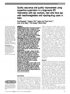
GENERIC PROCESS Vehicle testing is a very difficult task because numerous issues can prevent a validation of the model or, even worse, cause a spurious validation with erroneous data. These problems, in addition to test procedure, mainly include sensor accuracy, which can be affected by a host of factors, among which are electro-magnetic compatibilities, filtering, environmental conditions (e.g., temperature, humidity), vibrations, and software bugs, among others. To set an achievable goal for the vehicle modeling, one needs to first quantify uncertainties related to test measurements. ANL has been conducting very extensive testing of advanced vehicles, both from the point of view of instrumentation [13] and number of tests. Because of the large amount of data, a generic process is necessary to automatically generate reports that will allow engineers to quickly analyze data quality. This process, as shown in Figure 1, is based on five steps, each of them being described in detail in the following paragraphs. The goal of this process is to:
Automatically realign the data when different sources are used (e.g., emission bench, dynamometer). Select the proper sensor when the same parameter can be measured/recorded from different sources. Quantify the uncertainty of each sensor by comparing its values with measured or calculated parameters by using powertrain equations.
4- Calculate Effort/Flow Based on Sensors
5- QA Level 3: Sensor & Calculation Comparison
Figure 1: Generic Data Quality Analysis Process IMPORT DATA INTO PSAT The first step of the data quality analysis is the cornerstone of the process as it allows each sensor to be renamed and rescaled following PSAT nomenclature. On the basis of a nomenclature defined with the APRF testing team, the names and units of each sensor are read from the text file so they can be grouped by categories in the Graphical User Interface (GUI) “variable list,” as shown in Figure 2. The first time a test for a specific vehicle is loaded, each sensor has to be renamed, rescaled, or deleted. For example, a sensor named “Engine Speed,” measured in RPM, would be renamed “eng_spd_out_test” with units in “rad/sec.” Once the selections are completed for the entire list of sensors, the template is saved and can be reused when analyzing the next test for the same vehicle. Using the same PSAT nomenclature and units allows us to reuse the post-processing tools developed for simulation purposes to calculate parameters (e.g., energy, efficiencies). The only difference is that test data names end with “test,” whereas simulations end with “simu.” In the final step, each parameter is imported into Matlab.
Figure 2: PSAT Import Data Graphical User Interface AUTOMATED TIME ALIGNMENT As in most cases, data are collected from different data acquisition tools, and so it is often necessary to timealign the data to perform a more accurate analysis. An automated routine was developed in Matlab to minimize the difference between signals. The major issue is selecting the signals to be minimized. Even if it is preferable to use duplicated signals (e.g., vehicle speed from sensor or On-Board Diagnostic [OBD]), it is sometimes not possible. In that case, signals that should be highly correlated are selected (e.g., engine torque and emissions). Figure 3 compares two engine speed signals from different sources (sensor and OBD) after being realigned. QA LEVEL 1 – INDIVIDUAL SENSOR EVALUATION Figure 3: OBD and Sensor after Alignment The first level of quality analysis is used to visually check the range of the signals. For example, as shown in Figure 4, engine temperature should be maintained within a pre-defined range. During this step, a series of plots is defined for each parameter. This file can then be reused for any other test.
our signal with vehicle network data. Because of the slow frequency of the OBD (1 Hz), our sensor was selected for the analysis, and both OBD signals were deleted. Once each signal has been visually checked, signal accuracy has to be quantified. By using correlation, different sensors can be compared. As shown in Figure 6, both motor and wheel speeds are validated from their 2 high correlation (R >0.99). Other plots are also used to calculate the instantaneous absolute and relative errors between the signals. This plots are, however, more difficult to analyze because a slight misalignment can lead to significant differences. Until some more research is done in this area, average values are used, as shown in Table 2. Figure 4: Validation of Engine Temperature Range QA LEVEL 2 – SENSOR COMPARISON The goal of this step is to compare different signals for the same component. As shown in Figure 5, three signals were available for the engine speed during our testing of the 2004 Prius. Two were from the OBD (eng_spd_out_OBD_test and eng_spd_target_test), and the last one was from our own sensor (eng_spd_out_test). This example allowed us to validate
Figure 6: Correlation between Motor and Wheel Speeds The above examples demonstrated how the accuracy of each signal would be analyzed by using plots and statistical analysis. A summary of the duplicated sensors for the 2004 Prius and their accuracies is presented in Table 2. Note that the report is automatically compiled with the plots and summary tables from PSAT GUI. Also note that the process highlighted the quality of the data with high correlation values for the vehicle and engine speeds. The lower correlation value of the battery voltage between sensor and OBD raises the question of which Figure 5: Comparison between Three Engine Speed Sensors Parameter Vehicle Speed (Sensor) Engine Speed (Sensor) Direct Fuel Measurement (Sensor) Battery Voltage (Sensor) Boost Output Voltage (Sensor)
OBD OBD Fuel calculated from emissions
Correlation Absolute Difference Relative Difference Coefficient 0.34832 [m/s] -0.15053 [m/s] 0.99 3.5427 [rad/s] -0.43695 [rad/s] 0.98 4.4183e-005 [kg/s] -0.48228 [kg/s] 0.96
OBD OBD
7.3736 [volt] 10.4173 [volt]
Compared to
0.048639 [V] -0.010466 [V]
Table 2: Evaluation of Sensor Uncertainties — Summary Example
0.9 0.96
sensor to use. The calculated values from the table are generated from the correlation equations. To make the final decision, additional parameters may need to be calculated, in addition to the measured/recorded ones. CALCULATION OF MISSING EFFORT/FLOW It is impossible to measure the effort and flow of each component because of (1) time and cost constraints and (2) hardware accessibility. As previously discussed, it is possible to calculate parameters from measured/recorded signals to evaluate their accuracy. Mathematical equations can be used to calculate the effort and flow at the input/output of each component. These parameters can then be used to calculate the power, energy, and efficiency. For example, the final drive rotational input and output speeds can be calculated from the wheel speed. Indeed, the final drive output speed is identical to the wheel input speed. The final drive input speed can then be calculated by using the final drive ratio. QA LEVEL 3 – COMPARISON BETWEEN SENSOR AND CALCULATIONS Once all the calculations are done, a thorough comparison can be performed between calculated and measured parameters. During the testing of the 2004 Prius, the wheel torque (TWheel) and engine torque (TEngine) were measured, and the motor torque (TMotor) was recorded from the OBD. As shown in Figure 7, the motor torque can be calculated by using the following steady-state equations:
TMotor
TWheel TRing Ratio Final _ Drive
(1)
Nr Ns Nr
(2)
With TRing TEngine *
Figure 7: Comparison between Motor Torque from OBD and Calculation Using Measured Engine and Wheel Torques The example below is based on the Willis speed equation for a planetary gearset:
WMotor * Nr WEngine * ( Nr Ns) WMotor 2 * Ns
In Figure 8, both motor speeds are recorded from the OBD while two signals are used for the engine speed (from sensor and OBD). The comparison highlights a problem during transients because of the slow frequency of the OBD signals. We notice that the error is minimized when all OBD signals are used simultaneously. On the basis of this result, the motor speed was calculated from the vehicle speed, and the second motor (generator) speed was calculated from the Willis equations as the engine speed was previously validated during the QA Level 2.
with Nr and Ns the number of teeth at the ring and the sun. By comparing the OBD motor torque with the steadystate value based on measured engine and wheel torques, both sensors can be compared. In that case, we have to consider the uncertainties related to the calculation as (1) the equations are based on the steady-state value and (2) the OBD values have slower frequency. The last step of this example is to decide which motor torque signal should be used for the analysis. In this case, we decided to calculate the parameter on the basis of measured signals rather than using a slower recorded signal.
(3)
Figure 8: Verification of Willis Speed Equations Reveals Problem during Transients
In the following example, we compare the calculated wheel torque sensor with the value calculated from the vehicle acceleration signal and an assumed increase in static mass due to component inertia, as shown below.
TWheel FVeh _ out * Wheel _ Radius
(4)
With
Fveh _ out MassVeh * AccelVeh * Percent _ Inertia
(5)
Figure 9 validates the equations used and the sensors. One could note that this methodology could lead to minimizing the number of sensors in the vehicle. Indeed, for future vehicle testing, the number of sensors could be minimized if using the equations is proven acceptable.
With
2 FVeh _ Loss A B * Vveh C * Vveh
(7)
with A, B, and C the dynamometer coefficients. Figure 10 validates the operation of the dynamometer. A document including the plots and the summary table (Table 3) is automatically generated from the PSAT GUI. In addition to the absolute difference, the range of the test signals is also provided. The results below allowed us to conclude that the signals were all valid, considering the small absolute difference compared to the range.
Figure 9: Validation of Wheel Torque Using Measured and Calculated Values
Figure 10: Validation of Vehicle Force Using Measured and Calculated Values
The last example relates to vehicle force, the first one being measured and the second one calculated by using the following equations:
At this point, we are able to only keep the signals that have been labeled as “accurate.” The selection process is described in the following paragraph.
Fveh _ in Fveh _ out Fveh _ loss
Components Vehicle Wheel Wheel Engine Engine Motor 1 Motor 1 Motor 2 Motor 2 ESS Boost Converter
Calculated signal force speed torque torque (1) torque (2) speed torque speed torque SOC Current out
(6)
Absolute Difference with test -249.2 [N] 1.5 [rad/s] 1.7 [Nm] 5.6 [Nm] 7.6 [Nm] 5.7 [rad/s] 5.0 [Nm] -16.6 [rad/s] 1.9 [Nm] -0.1 [[0,1]] 1.9 [amps]
Range of test signal [-3197 ; 18585] [N] [-0.2 ; 83] [rad/s] [-832 ; 1399] [Nm] [-25 ; 120] [Nm] [-25 ; 117] [Nm] [-1.05 ; 343] [rad/s] [-192 ; 215] [Nm] [-592 ; 811] [rad/s] [-32.6 ; 7.8] [Nm] [0.5 ; 0.77] [[0,1]] [-49 ; 126] [amps]
Table 3: Evaluation of Uncertainties between Measured and Calculated Parameters — Summary Example SIGNAL SELECTION Parameters were deleted for four main reasons:
1. Signals with low correlation coefficients or that appeared suspicious from the visual check (e.g., speed higher than maximum literature values) were deleted. 2. When several sources were available for the same parameters, the sensor installed by test engineers was preferred to OBD or dynamometer signals. 3. To ensure consistency in the mathematical relationships, both electric machine speeds from OBD were not kept. Indeed, we noticed that the Willis equations were not satisfied during transients because of the large sample and delay from the OBD signals with the engine speed. 4. Signals from the OBD were not recognized (issue with units or with meaning).
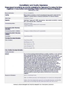
UNDERSTANDING THE CONTROL STRATEGY GENERIC PROCESS The final template is used to import the validated sensors into Matlab by using PSAT nomenclature. The process used to understand control strategies, shown in Figure 11, is similar to that used for the analysis of data quality. A calculation file is used to define the missing effort and flow of each component, and then a series of pre-defined plots is used to understand vehicle behavior. The analysis is used to develop the control strategy in PSAT where an HTML report is automatically generated. Once the calculation is performed, one has also the ability to export the data back to an EXCEL file so they can be analyzed by other persons.
result of previous PSAT validation using 1999 and 2001 models tested at ANL’s APRF. The Prius supplies the necessary road demand to the wheels under the constraints of operating the engine close to its most efficient curve (as shown in Figure 12) while sustaining the battery pack SOC. The operating point of the engine is chosen as follows. A desired vehicle road demand power is calculated by using the vehicle speed and accelerator pedal position. Then, the battery SOC is used to calculate a battery power demand. Both power demands are added to produce the total vehicle demand. If the total vehicle demand is greater than a threshold, the Prius turns the engine ON; otherwise, it will operate in EV mode until the SOC is low enough to create a battery power demand of sufficient magnitude to turn the engine ON. Once the engine is ON, the desired power (wheel + SOC regulation) is set to the engine power. The vehicle controller then tries to maximize the system efficiency, in most cases by operating the engine close to its best efficiency curve. Knowing the engine speed, the vehicle controller then determines the desired generator speed. The generator’s controller converts the error between the desired and actual generator speeds into the desired generator torque. By using the desired generator torque, the engine torque, and the torque demand at the wheels, the desired motor torque is calculated. A motor assist during acceleration is implicit in this calculation since the wheel torque demanded during acceleration is greater than the maximum torque of the engine.
Final template Calculation
Import data
m.file
Control Strategy Analysis
Validation
XLS
e-report
Figure 11: Generic Process Used to Understand Control Strategies TOOLS DEVELOPED The control strategy philosophy of the power split system is well documented in the literature and as a
Figure 12: Engine Operating Points on UDDS Cycle
Consequently, the main goal of an HEV control strategies validation is to understand:
POWERTRAIN MODEL VALIDATION GENERIC PROCESS
Why the engine turns ON, When/How to regulate the battery SOC, and The repartition between mechanical regenerative braking.
and
Understanding the control strategies of HEVs requires innovative tools, especially when considering power split systems, such as those in the Toyota Prius. To accelerate the process, several plots have been defined. Figure 13, for example, shows the repartition of the engine power during an UDDS driving cycle.
Once the control strategy philosophy has been understood from the test data, several steps are still necessary to validate the model, as described in Figure 15. First, each component has to be modeled, including the engine, the electric motors, the battery, and the driveline. As in most cases, some of the models were developed on the basis of the manufacturer’s literature [12, 14, 15, 16], while others were developed through testing. In this case, the battery data were provided by Idaho National Laboratory.
Component Model Steady-State Validation Low Transient Cycles
SOC1 SOC2
High Transient Cycles Figure 13: Engine Power Distribution during UDDS Cycle Figure 14 shows the distribution of the battery current during regenerative events.
SOCn
Figure 15: Generic Model Validation Process Once the vehicle powertrain models are defined, the validation process begins with the steady-state cycles. We then increase the difficulty of the cycles, going from low transients (e.g., Japan 1015, NEDC) to high transients (e.g., UDDS, HWFET, US06). CONTROL STRATEGY The generic State Diagram representation of the control strategy is shown in Figure 16.
Figure 14: Battery Current Distribution during Regenerative Events
On the basis of the test results, the engine will be turned ON based upon (1) vehicle speed, (2) engine power demand threshold, and (3) maximum available battery power. The engine power demand is based on the wheel torque demand adjusted on the basis of the battery SOC. Intermediate states (Eng_On_MinTime and Eng_Off_MinTime) were used to maintain the engine in the “Eng_Off” or “Eng_On” states to avoid oscillations. Similarly, every threshold will only be valid after a specified time.
CONCLUSION A generic process allowing automated data quality analysis and facilitating vehicle model validation has been presented. In addition to significantly accelerating the validation process, the methodology allows an indepth analysis of test sensor uncertainties and the vehicle control strategy. This generic process can be applied to all vehicle configurations. Once developed, the process allowed us to analyze test data uncertainties within minutes versus days and validate the Toyota Prius 2004 PSAT vehicle model. However, additional work needs to be done to characterize the acceptable test and validation errors. The report compares measured and calculated signals from test data, but it does not yet take into account the cumulative uncertainties of the signals.
ACKNOWLEDGMENTS
Figure 16: State Diagram Representation of the Control Strategy
This work was supported by the U.S. Department of Energy, under contract W-31-109-Eng-38. The authors would like to thank Lee Slezak of DOE, who sponsored this activity.
REFERENCES The “Eng_On” state is used to select the proper state in the “Propel Control,” and the “Electric Vehicle Mode” is used when the engine is OFF. Within all of the states of “Propel Control,” two states are defined: one for normal operating mode and the other when the maximum battery power is achieved (either for charging or recharging). If the engine is OFF, it will be turned ON. Otherwise, the engine will not be operated close to its best efficiency curve to be able to achieve the main goal of the controller: follow the vehicle trace. SIMULATION RESULTS An example of the simulation results is shown in Figure 17 for the Japan 1015. As for any validation, we started by reproducing the operating conditions of the components. Indeed, once the simulated engine ON/OFF and the effort and flow of each component match the test data, both fuel economy and battery state-of-charge are a natural consequence. As can be seen in the figure, the differences between the measured and simulated values are within the test error. The difference between the SOC from OBD and simulation comes from the algorithm used to calculate SOC in the model, which is based on 6.5-Ah capacity. The algorithm used in the vehicle is different from the one used in simulation. As discussed previously, the report is automatically generated after the simulation. One should also note that several test data can be compared by using the same process to evaluate testto-test variability.
1. http://www.eere.energy.gov/vehiclesandfuels/ 2. Argonne National Laboratory, PSAT (Powertrain Systems Analysis Toolkit), http://www.transportation. anl.gov/. 3. Rousseau, A.; Sharer, P.; and Besnier, F., "Feasibility of Reusable Vehicle Modeling: Application to Hybrid Vehicles," SAE paper 2004-011618, SAE World Congress, Detroit, March 2004. 4. Rousseau, A.; Pagerit, S.; and G. Monnet, “The New PNGV System Analysis Toolkit PSAT V4.1 — Evolution and Improvements,” SAE paper 01-2536, Future Transportation Technology Conference, Costa Mesa, Calif., August 2001. 5. The Mathworks, Inc., Matlab Release 14, User's Guide, 2005. 6. Sharer, P.; Rousseau, A.; Pagerit, S.; and Wu, Y., "Impact of FreedomCAR Goals on Well-to-Wheel Analysis," SAE paper 2005-01-0004, SAE World Congress, Detroit, April 2005. 7. Pagerit, S.; Rousseau, A.; and Sharer, P., “Global Optimization to Real Time Control of HEV Power Flow: Example of a Fuel Cell Hybrid Vehicle,” 20th International Electric Vehicle Symposium (EVS20), Monaco, April 2005. 8. Rousseau, A.; Sharer, P.; Pagerit, S.; and Das, S., “Trade-off between Fuel Economy and Cost for Advanced Vehicle Configurations,” 20th International Electric Vehicle Symposium (EVS20), Monaco, April 2005.
SOC (%) 0.62
Cumulated Fuel Consumption (kg) TEST
0.1
0.6
0.08
TEST
0.06 0.58 0.04 SIMU
0.02
0.56
0
SIMU 0.54
-0.02 0
0.52 0
100
200
300
400
500
600
700
Time (s) 100
200
300
400 Time (s) Difference SOC (%)
500
600
700 Difference Cumulated Fuel Consumption (%)
2
5
0
0.71%
0
-1.24% -2
-5
-4 -6
-10
-8 -15 -10 -12 0
100
200
300
400
500
600
700
-20 0
100
200
300
Time (s)
400
500
600
700
600
700
Time (s)
Engine Torque (Nm)
Wheel Torque - Driver Demand (Nm)
120
600
100
SIMU
400
80 200
60 40 20 0 -20
0 -200
Number of Engine Starts Test : 10 Simu : 10
-40 0
100
200
-400
300
400
500
600
700
-600 0
100
200
Time (s)
300
400
500
Time (s)
Figure 17: Summary of Prius 2004 Validation – Example for Japan 1015
9. Pasquier, M.; Rousseau, A.; and Duoba, M., "Validating Simulation Tools for Vehicle System Studies Using Advanced Control and Testing Procedures,” 18th International Electric Vehicle Symposium (EVS18), Berlin, Germany, October 2001. 10. Rousseau, A., and Pasquier, M., “Validation of a Hybrid Modeling Software (PSAT) Using Its Extension for Prototyping (PSAT-PRO),” Global Powertrain Congress, Detroit, June 2001. 11. Rousseau, A., and Larsen, R., 2000, “Simulation and Validation of Hybrid Electric Vehicles Using PSAT,” Global Powertrain Congress, Detroit, June 2000. 12. Toyota, “Development of New-Generation Hybrid System THS II - Drastic Improvement of Power Performance and Fuel Economy,” SAE paper 200401-0064, SAE World Congress, Detroit, March 2004. 13. Bohn, T., and Duoba, M., “Implementation of a NonIntrusive In-Vehicle Engine Torque Sensor for
Benchmarking the Toyota Prius,” SAE paper 200501-1046, SAE World Congress, Detroit, April 2005. 14. Toyota, “Prius 2004 New Car Features.” 15. Toyota, “Development of a New Battery System for Hybrid Vehicles,” 20th International Electric Vehicle Symposium (EVS20), Monaco, April 2005. 16. Toyota, “Development of Hybrid Electric Drive System Using a Boost Converter,” 20th International Electric Vehicle Symposium (EVS20), Monaco, April 2005.
CONTACT Aymeric Rousseau (630) 252-7261 E-mail:
[email protected]
APPENDIX TMotor
Motor torque (Nm)
TWheel
Wheel torque (Nm)
TRing
Ring torque (Nm)
TEnginer
Engine torque (Nm)
Nr
Number of teeth of the ring
Ns
Number of teeth of the sun
RatioFinal_Drive
Final Drive Ratio
Wheel_Radius
Wheel radius (m)
WMotor
Rotational Sped of the motor (rad/s)
WMotor2
Rotational Sped of the second motor (rad/s)
WEngine
Rotational Sped of the engine (rad/s)
MassVeh
Vehicle test mass (kg)
AccelVeh
Vehicle Acceleration (m/s2)
Percent_Inertia
Percentage of additional vehicle weight due to inertia
FVeh_in
Vehicle force before losses (N)
FVeh_Out
Vehicle force after losses (N)
FVeh_loss
Vehicle force losses (N)
A,B,C
Dynamometer coefficients (also called f0, f1, f2)