SAE TECHNICAL PAPER SERIES
2000-01-1294
Integrating Design and Virtual Test Environments for Brake Component Design and Material Selection Sydney G. Roberts and Terry D. Day Engineering Dynamics Corporation
SAE 2000 World Congress Detroit, Michigan March 6-9, 2000 400 Commonwealth Drive, Warrendale, PA 15096-0001 U.S.A.
Tel: (724) 776-4841 Fax: (724) 776-5760
The appearance of this ISSN code at the bottom of this page indicates SAE’s consent that copies of the paper may be made for personal or internal use of specific clients. This consent is given on the condition, however, that the copier pay a $7.00 per article copy fee through the Copyright Clearance Center, Inc. Operations Center, 222 Rosewood Drive, Danvers, MA 01923 for copying beyond that permitted by Sections 107 or 108 of the U.S. Copyright Law. This consent does not extend to other kinds of copying such as copying for general distribution, for advertising or promotional purposes, for creating new collective works, or for resale. SAE routinely stocks printed papers for a period of three years following date of publication. Direct your orders to SAE Customer Sales and Satisfaction Department. Quantity reprint rates can be obtained from the Customer Sales and Satisfaction Department. To request permission to reprint a technical paper or permission to use copyrighted SAE publications in other works, contact the SAE Publications Group.
All SAE papers, standards, and selected books are abstracted and indexed in the Global Mobility Database
No part of this publication may be reproduced in any form, in an electronic retrieval system or otherwise, without the prior written permission of the publisher. ISSN 0148-7191 Copyright © 2000 Society of Automotive Engineers, Inc. Positions and opinions advanced in this paper are those of the author(s) and not necessarily those of SAE. The author is solely responsible for the content of the paper. A process is available by which discussions will be printed with the paper if it is published in SAE Transactions. For permission to publish this paper in full or in part, contact the SAE Publications Group. Persons wishing to submit papers to be considered for presentation or publication through SAE should send the manuscript or a 300 word abstract of a proposed manuscript to: Secretary, Engineering Meetings Board, SAE.
Printed in USA
2000-01-1294
Integrating Design and Virtual Test Environments for Brake Component Design and Material Selection Sydney G. Roberts and Terry D. Day Engineering Dynamics Corporation Copyright © 2000 Society of Automotive Engineers, Inc.
environment, the designer may specify the characteristics of the vehicle, choose the brake system properties, and then subject the vehicle to any series of user defined maneuvers, such as stopping distance tests or split-mu braking.
ABSTRACT A new, systematic approach to the design-evaluation-test product development cycle is described wherein the vehicle design and simulation environments are integrated. This methodology is applied to brake mechanical design and material selection. Time-domain computations within a vehicle dynamic simulation environment account for brake and lining geometry and material properties, actuator properties, and temperature effects. Two examples illustrate the utility of this approach by examining: the effect of varying hydraulic cylinder diameter on passing federally mandated stopping distance tests, and the effect of S-cam actuator adjustment on the performance of air brakes on a tractortrailer. The simulation results are compared with experimental vehicle stopping distance tests to assess the validity of the simulations. Implementing virtual testing early in the product development cycle has the potential to shorten development time, reduce the risk of failure during expensive physical testing, and increase the overall product quality.
By integrating the design and virtual test environments in this way, the designer can quickly and easily perform parametric studies by varying any one of the many brake system variables. Complex test matrices can be constructed that would not be practical in physical testing. Tests that are not possible on physical proving grounds due to lack of facilities or danger of the maneuver can also be simulated. By performing tests on the digital proving ground throughout the design process, one can have greater confidence that a design will succeed on the actual physical proving ground.
BRAKE DESIGNER DESCRIPTION The HVE Brake Designer is a commercially available time domain simulation model that interfaces directly with validated vehicle dynamics simulation models (EDVSM and EDVDS). Brake geometric and mechanical characteristics and component material properties are user-defined for a variety of standard brake types. The following brake types may be used in any combination on passenger vehicles and tractor-trailers:
INTRODUCTION Maximizing quality within cost, time, and space constraints is the goal of an effective design process. This is a particularly challenging task in vehicle design where it is common for different teams to design individual components that must function in harmony with components designed by others. Allowing the performance of a single component to be evaluated within a total vehicle model can therefore enhance the design process.
• Disc Brake • Duo-Servo Drum Brake • Duplex Drum Brake • Single Piston Drum Brake • Dual Piston Drum Brake • S-Cam Drum Brake
With this goal in mind, the HVE Brake Designer was created to aid designers in choosing brake types, dimensioning brake parts, and choosing friction materials. HVE, Human-Vehicle-Environment, is a computer simulation environment that has been validated for the dynamic simulation of passenger vehicle, truck, and combination vehicle behavior (Day, 1993; Day, 1997; Day, 1999). Within this integrated design/test
• Single Wedge Drum Brake • Dual Wedge Drum Brake For each brake type, the user must prescribe specific geometric and material properties to the brake actuator, rotor/drum, brake shoes, and friction materials (Figure 1 and Figure 2). From these inputs, the simulation model
1
Stroke factor is used to account for the loss in actuation force at increased levels of stroke (Figure 3).
computes brake factor, actuation factor, and, ultimately, brake torque at user-defined timesteps. Current brake torque is then used by the vehicle dynamics model in the simulation of vehicle performance. Input Actuator properties Rotor/drum geometry Rotor/drum material properties Lining geometry Lining material properties Lining friction properties Output Brake Factor (BF) - the ratio of lining friction force to brake actuation force Actuation Force (AF) - force produced by the brake actuation device (lb) Brake Torque (BT) - torque applied by the brake system about the wheel center (in-lb) BT = BF × TR × AF × SF
where TR = radius of brake friction force (in) SF = (Stroke Factor) percentage of reduction in actuation force normally resulting from excessive air chamber stroke MECHANICAL ANALYSIS – Equations for brake torque for the eight different brake types are given by Limpert (1992). Disc brakes For disc brakes, the free body analysis is relatively simple and is presented below. BF = 2 × µ TR = (Ro + Ri ) / 2
AF = (Pline − Ppushout ) × Apiston × N pistons × ηmechanical SF = 1
Drum brakes The free body analysis of drum brakes is straightforward yet long, so the derivation will be left to the interested reader. The equations of brake force for leading and trailing pinned and abutted shoes are appropriately combined to form the equation for total brake force for each of the seven drum brake types. Example 2 will illustrate the importance of considering the chamber stroke for a drum air brake with an S-cam actuator.
Figure 1.
2
Actuator, drum, and lining data are input by the user for a model of an S-cam actuated drum brake.
Stroke Factor
Figure 2. Drum and lining material properties are input by the user for a model of an S-cam drum brake.
1.0
H! = Work × Rate
0.8
H! = Brake Torque × Wheel Spin Velocity
0.6
This energy is transmitted into the brake linings and rotor/ drum through conduction, stored through capacitance, and lost to the atmosphere through convection. Radiant heat transfer is not considered because of its negligible effect on the system at normal operating temperatures.
0.4 0.2 0.0 0.0
0.5
1.0
1.5
2.0
2.5
Because of geometric differences between disc and drum brakes, the model of heat flow varies slightly between the two cases. We will present the formulation for the drum brake, but the model for the disc brake is set up similarly.
3.0
Brake Stroke (in) Figure 3.
Stroke Factor is strongly dependent on Brake Stroke (slack adjustment) for an air brake with S-cam actuator.
A lumped mass model consisting of 10 interior drum nodes, 1 interior lining node, and 1 each lining and drum exterior nodes was developed. Temperature is calculated at each of these 13 nodes. The First Law of Thermodynamics for the system may be expressed as:
TEMPERATURE ANALYSIS – During braking, the vehicle’s kinetic energy is converted into heat energy at the pad/lining and rotor/drum interfaces. This input of heat energy into the brake assembly components is then dissipated to the atmosphere through both conduction and convection.
[M ]
This transfer of energy is modeled using a lumped mass method adapted from MacAdam, et. al. (1980).
dT dt = [S ] [T ] + [C ] T L / D + [D ] T A
where
Modeling Technique – The rate of work ( H! ) into the system is proportional to brake torque and wheel spin velocity.
[M]
= Capacitance matrix
dT dt = Thermal Rate matrix
3
[S]
= Internal Temperature Coefficient matrix
Thermal Capacitance Matrix
[T]
= Temperature matrix
Rotor/drum
[C]
= Boundary Conductivity matrix
TL/D
= Interface Temperature
[D]
= Boundary Convectivity matrix
TA
C D = C pD ρ D V
where
= Ambient Temperature
The matrix equation is solved for the node temperatures at each integration timestep. The specific temperatures affecting brake system performance are T5 (interior drum), TL/D (interface), and T12 (interior lining).
)
V =
(Drum)
V = π DD W L x D
Lining C L = C pL ρ L VL
Model Inputs – Inputs to the lumped mass model are divided into geometric, material, and temperature variables.
where
Drum inner diameter (drum) (DD) Drum thickness (drum) (xD) Lining width (drum) (WL) Lining thickness (xL) Rotor inner and outer diameters (disc) (Di, Do) Rotor thickness (disc) (xR) Pad included angle (disc) (γL) Lining inner and outer radii (RLi, RLo)
(D
γ π
(Rotor)
VL =
(Drum)
α pri + α sec VL = 360
Geometric
o
1440
2
)
− Di 2 x L
π DD W L x L
where
αpri
= arc length of primary shoe
αsec = arc length of secondary shoe The 13 x 13 diagonal capacitance matrix [M] is formed using the rotor/drum and lining capacitance coefficients.
Material Rotor/drum specific heat (CpD) Rotor/drum density (ρD) Rotor/drum material conduction coefficient (kD) Rotor/drum static and velocity-dependent convection coefficients (H0D, H 1D) Lining specific heat (CpL) Lining density (ρL) Lining material conduction coefficient (kL) Lining static and velocity-dependent convection coefficients (H0L, H 1L)
2 21 C D [M ] =
Temperature Ambient temperature (TA) Initial rotor/drum temperature (T0D) Initial pad/lining temperature (T0L)
• • • 2 CD 21 1 CD 21 2 CL 3
Internal Temperature Coefficient Matrix
Model Outputs – The output temperatures that are of particular interest in determining brake system performance are listed below. Alphabetical subscripts refer to the component or location.
Rotor/Drum KD =
Lining External Surface Temperature (TLS) Lining Internal Temperature (TL) Interface Temperature (TL/D) Drum Internal Temperature (TD) Drum External Temperature (TDS)
k D AD xD
where KD = Conductivity coefficient of rotor/drum AD = Heat transfer area of rotor/drum
Equations
=
Lining/Drum Interface Temperature TL / D =
(
π 2 2 Do − Di xR 4
(Rotor)
H! + 21 K D T D1 + 3 K L T D10
π 4
(D
2 o
− Di 2
= π DD W L
21 K D + 3 K L
4
)
(Rotor) (Drum)
1 CL 3
Solution Procedure
Lining KL =
k L AL
[S ′] = [M ]−1 [S ]
xL
[C ′] = [M ]−1 [C ]
where
[D ′] = [M ]−1 [D]
KL = Conductivity coefficient of lining solve for
AL = Heat transfer area of lining =
γ π 1440
(D
2 o
α pri + α sec = 360
)
(Rotor)
π DD W L
(Drum)
− Di 2
dT dt = [S ′] [TPr ev ] + [C ′] T L / D + [D ′] T A
where TPrev = Temperature at previous timestep The internal temperature matrix is then computed at each integration timestep.
Convection Coefficients Rotor/Drum
(
H D = H 0D + H 1D V
)A
[T ] = dT dt
D
∆t + [TPrev ]
where
where
HD = Convectivity matrix coefficient for rotor/drum
∆t = Integration timestep
V
As mentioned previously, brake system performance is heavily influenced by drum and lining internal temperatures and lining/drum interface temperature. Lining friction, and thus brake torque, is a function of lining/drum interface temperature. Within the HVE Brake Designer, the user is able to define the relationship between lining friction and temperature across the full range of operating temperatures. Increasing brake drum temperature also has the effect of increasing drum diameter and requiring an increase in brake stroke for air brake systems with S-cam actuators. This increase in brake stroke causes a decrease in actuation factor (Figure 3). While this decrease is small for properly adjusted brakes, it can become catastrophically large when the initial stroke is near the knee in the stroke vs. actuation factor curve.
= Vehicle linear velocity
Lining
(
H L = H 0L + H 1L V
)A
L
where HL = Convectivity matrix coefficient for lining The 13 x 13 internal temperature coefficient matrix [S] is formed using the rotor/drum and lining conductivity and convectivity coefficients.
[S ] = − 63 21 KD KD 2 2 21 K D − 21K D 21 K D 2 2 • • • • • • − 63 21 K K K 21 D D D 2 2 21K D − 21K D − HD −9 3 KL KL 2 2 −3 3 KL KL − HL 2 2
DESIGN AND TESTING ENVIRONMENT INTEGRATION The Brake Designer is incorporated into two HVEcompatible physics models used to simulate vehicle behavior: one for passenger vehicles (EDVSM) and one for articulated vehicles (EDVDS). HVE provides the graphical simulation environment while the physics models govern vehicle behavior.
Internal Temperature Matrix
[T ] = [T1
T2 T3 T4 T5 T6 T7 T8 T9 T10 T11 T12 T13 ]
Physical properties describing each vehicle are input by the user. These include brake, suspension, drive train, tire, and crush stiffness characteristics. Additionally, a 3dimensional body image is used to visualize the model. Vehicle color, reflectivity, glass transparency, etc. may all be edited.
T
Boundary Condition Matrix
[C ] = [21K D
0 0 0 0 0 0 0 0 0 0 3K L
0]
T
Boundary Condition Matrix
[D ] = [0
0 0 0 0 0 0 0 0 0 HD
0 HL ]
Within HVE, the user is able to construct 3-dimensional environments with which vehicles interact. Objects in these environments can include roads, curbs, medians,
T
5
as single effectiveness braking, the simulation of wear and fatigue is not incorporated into the Brake Designer model.
guardrails, embankments, light and telephone poles, trees, etc.. For each object, the user must define physical properties that govern both appearance and mechanical properties. For instance, one can model an icy patch of road by changing the friction properties and reflective properties of one section of the road surface. Other objects may be entered with only visual, and not physical, properties; common examples include buildings, street signs, and trees.
Initial conditions and driver controls from an average of six actual tests were input into the simulation model. Ambient temperature was 57 deg F. Test weight including equipment and occupants was 4890 lbs. Initial brake temperatures were 180 and 182 deg F for the 30 mph and 60 mph tests, respectively.
Human passenger and pedestrian dummies may also be included. Belt restraints may be added to vehicle passenger dummies. Size, joint characteristics, and ellipsoid/contact surface stiffnesses are all user editable.
The simulations were started with the vehicles traveling in neutral gear at 1 mph over the test speed. No brake or throttle were applied. When the vehicle slowed to the test speed, brake pedal force was increased linearly from zero to the average pedal force (listed in Table 2) over 0.25 seconds. This pedal force remained constant until the vehicle slowed to 0.50 mph, at which point the simulation terminated.
Once the vehicle and environment have been defined, the user creates an event complete with vehicle initial conditions (positions and velocities) and optional driver controls, such as steering and braking. Environmental variables including time and date, temperature, and fog may also be selected. Models have been developed for special functions such as a tire blow-out (Blythe, 1998).
Table 2. FMVSS 105 Test and Simulation Results Average Pedal Force (lb)
HVE thus easily lends itself to parametric studies in which one vehicle, environment, or event variable is changed, and the effect of that change is quantified in vehicle performance. Two examples of parametric studies using the Brake Designer follow: changing hydraulic cylinder diameter of multi-purpose vehicle (MPV) disc brakes, and changing slack adjustment of tractor-trailer air brakes.
EXAMPLE 1: MPV HYDRAULIC DISC BRAKES: STOPPING DISTANCE The effect of brake cylinder diameter on passenger vehicle stopping distance was assessed by simulating a test of stopping distance (FMVSS 105) for a 1996 Ford Explorer, 2-door MPV (HS # 632072). The actual and simulated vehicles were equipped and loaded similarly. The vehicle had front and rear hydraulic disc brakes (dimensions in Table 1). The program EDVSM was used for this simulation.
Rear
Piston
Hydraulic Piston Diameter (in)
1.81
1.89
Rotor
Diameter (in) Thickness (in)
11.28 1.023
11.22 0.472
Pad
Width (in) Length (in) Thickness (in) SAE Code
1.717 5.354 0.390 EE
1.199 4.914 0.374 EE
30 mph Standard Test Simulation
< 150 31.9 31.9
24.0 23.0 18.0
65.0 56.8 58.8
60 mph Standard Test Simulation
< 150 64.6 64.6
23.0 23.4 22.2
242.0 191.8 184.5
For both the 30 mph and 60 mph first effectiveness braking test, simulated stopping distance was less than 4% different than actual stopping distance (Table 2). Average deceleration rates were also close, but underestimated, by the simulation. The Brake Designer model does not, however, currently include a model for anti-lock braking. While the variable proportioning model prevented lock-up of the rear wheels in the 60 mph test, the front wheels did lock-up. This condition violates the FMVSS 105 Procedures. Clearly, the anti-lock brake system on this vehicle is critical to proper braking performance at highway speeds. Inclusion of an anti-lock model into the Brake Designer and HVE is planned for future development.
Table 1. Disc Brake Dimensions Front
Average Stopping Deceleration Distance (ft/sec^2) (ft)
It is important to note that the entire time history of the applied brake pedal force was not available. In the actual tests, maximum brake pedal forces were 43.7 and 84.7 lbs for the 30 mph and 60 mph tests, respectively. Because it is not known at what point these forces were applied, no attempt was made to use them as input to the simulation model. If such high brake pedal forces were entered, increased average deceleration rates would be expected.
The first effectiveness test from standard FMVSS 105 was simulated in this example. Although FMVSS 105 specifies standards and procedures for repetitive as well 6
the bottom, we compared stopping distance and time for the vehicles making an emergency stop. The program EDVDS was used for this purpose.
Also critical to consider when comparing any simulated to actual test results is the fact that the simulation represents an idealized scenario. In this case, the brake components and tire/road interface are simulated as functioning perfectly. Likewise, the driver is simulated as applying perfectly steady pressure throughout the entire test. Both of these assumptions may not have matched actual test conditions. If more information were available, for instance precise tire/road friction values or pedal force as a function of time, it could have been input into the simulation.
In this example, a 1995 Freightliner FLD-120 with a sleeper towing a 45-ft box trailer is outfitted with wedge brakes on the front axle and S-cam brakes on the four other axles (dimensions in Table 3). The nominal friction coefficient was not adjusted for low and high temperatures. The center of gravity of a 42500-lb payload was placed such that maximum axel loads did not exceed allowable limits. This resulted in a total loaded vehicle weight of 73418 lb.
In order to demonstrate the usefulness of the brake designer for performing parametric studies, front piston diameter was decreased by 25% and the 60 mph braking test was repeated. In this case, the vehicle lost control at the end of the simulation (Figure 4). With the original configuration, the front wheels were locked for much of the simulation. With the reduced piston diameter, the front brake calipers applied a smaller brake torque for the same pedal force. Under these circumstances the front tires maintained lateral stability while the locked rear tires did not. Thus, the vehicle spun-out.
Table 3. Air Brake Designs and Dimensions Type Drum diameter x pad width (in) Air chamber diameter (in) Lining SAE code Friction coefficient
Wedge Type 20 15 x 3.5 9.0 FF 0.35
S-Cam Type 30 16.5 x 7 30.0 FF 0.35
Slack arm length was 6.5 inches. The vehicle began the descent with a forward velocity of 65 mph and the vehicle in the lowest allowable gear. Initial lining and drum temperatures were set to 100 deg F. Brake pedal force was applied such that vehicle speed stayed within 1 mph of the initial speed throughout the descent. In the air brake Brake Designer model, treadle valve pressure is equal to pedal force. After descending for 2.5 minutes, the grade became zero and the vehicle performed an emergency stop with 50 psi treadle pressure. The simulation was terminated when vehicle speed decreased to 2 mph.
Figure 4.
Using the formulations of the Grade Severity Rating System (Bowman, 1989), this truck should be able to safely stop after traveling this distance of 2.7 miles with brakes applied to maintain a speed of 65 mph. In fact, the maximum safe distance for this vehicle on this grade is over 4 miles.
Decreasing front piston diameter resulted in loss of control at the end of the braking maneuver.
Three simulations were run: with initial stroke set to 1.75, 2.00, and 2.25 inches. Recall that the knee in the stroke vs. actuation factor curve is at 2.00 inches.
Examples of additional tests from FMVSS 105 that are simulated using the HVE Brake designer, including spike stops and disabled component braking, are discussed by Canova (2000).
For initial stroke of 1.75 inches, a relatively constant velocity was maintained on the descent by applying a treadle valve pressure of 6.1 psi over 150 seconds. During this time, brake drum, lining, and drum-lining interface temperatures increased significantly, with lining temperature reaching over 325 deg F, and drum and drum-interface temperatures reaching over 450 deg F (Figure 5). Brake drum and drum-lining interface temperatures increase substantially faster than lining temperature for the first 60 seconds of the simulation. This is because the brake lining is a poorer heat conductor than the metal drum. As the simulation continues, the rate of increase in lining temperature
EXAMPLE 2: TRUCK AIR BRAKES: 6% GRADE DESCENT The drum brake temperature model was utilized in the simulation of a fully loaded tractor-trailer descending a straight 6% downhill grade in order to study the effect of brake adjustment on vehicle performance during an emergency stop. Using the concept used to develop the Grade Severity Warning System, in which a tractor-trailer must descend a grade and be able to make a safe stop at 7
increases. Because of rising brake temperature, treadle pressure required to maintain a constant speed was increased slightly. This resulted in an increase in brake stroke to 1.95 inches after 150 seconds.
5
Brake temperature increases during the descent were similar for the case with initial brake stroke of 2.00 inches. Brake stroke was 2.14 inches after 150 seconds.
3
4
Initial Stroke 1.75 2.00 2.25
2
Brake temperatures were lower, however, for the case with initial brake stroke of 2.25 inches. Lining, drum, and interface temperatures were 287, 387, and 395 deg F after 150 seconds. During this time brake stroke increased to 2.42 inches, and treadle valve pressure required to maintain a constant speed increased from 7.5 (at t = 0 seconds) to 11.8 psi (at t = 150 seconds).
1 0
Time
Figure 6.
These increases in brake temperature and brake stroke significantly affected vehicle performance during the emergency stop. The tractor-trailer with initial stroke of 1.75 inches stopped in 5.6 seconds and 311 feet. In the other two cases, the vehicles did not stop as effectively (Figure 6, normalized values). It took the tractor-trailer with 2.25 initial stroke 25.8 seconds and 1154 feet to stop.
Stopping time and distance normalized by values for initial stroke equal to 1.75 inches
During the stop, the properly adjusted vehicle achieved a brake torque of 97200 in-lb, where as in the cases of 2.00 and 2.25 initial stroke brake torque reached a maximum of 58200 and 14569 in-lb before abruptly fading (Figure 7). The emergency stop resulted in a temperature increase of 44 deg F for initial stroke of 1.75 inches compared to 27%, 36%, and 33% for initial stroke of 2.25 inches. 100000
1000
Initial Stroke 1.75
Drum
750
Brake Torque (in-lb)
Temperature (deg F)
Interface
Lining
500
250
75000
2.00 2.25
50000
25000
0
0
0
50
100
150
200
0
Time (seconds)
Figure 5.
Distance
50
100
150
200
Time (seconds)
Brake component temperatures rose steadily throughout the descent and rose sharply with during the emergency stop.
Figure 7.
8
Maximum brake torque and brake fade during the emergency stop were highly dependent on initial brake stroke.
CONCLUSIONS
REFERENCES
It has been demonstrated through two examples, a passenger car and a tractor-trailer, that integrating the design and testing environments in the HVE Brake Designer is a powerful tool for giving the engineer quantitative feedback regarding the effect of a single component design on entire vehicle performance.
1. Bowman, BL (1989) “Grade Severity rating system (GSRS) – Users manual.” FHWA-IP-88-015. 2. Blythe, W; Day, TD; Grimes, WD (1998) 3Dimensional simulation of vehicle response to tire blow-outs. SAE Paper No. 980221. 3. Canova, JH (2000) Vehicle design evaluation using the digital proving ground. SAE Paper No. 2000-010126. 4. Day, TD (1993) A computer graphics interface specification for studying Humans, vehicles and their environment. SAE Paper No. 930903. 5. Day, TD (1997) Validation of the EDVSM 3dimensional vehicle simulator. SAE Paper No. 970958. 6. Day, TD (1999) Differences between EDVDS and Phase 4. SAE Paper No. 1999-01-0103. 7. U.S. Department of Transportation, NHTSA (1992) Laboratory test procedure for FMVSS 105 – Hydraulic brake systems. TP-105-02. 8. Johnson, WA; DiMarco, RJ; Allen, RW (1982) “The development and evaluation of a prototype grade severity rating system.” FHWA/RD-81/185. 9. Limpert, R (1992) “Brake Design and Safety.” Society of Automotive Engineers. Warrendale, PA. 10. MacAdam, CC; Fancher, PS; Hu, GT; Gillespie, TD (1980) “A computerized model for simulating the braking and steering dynamics of trucks, tractorsemi-trailers, doubles, and triples combinations – Users’ manual.” Report No. UM-HSRI-80-58, HSRI, University of Michigan.
As with all modeling, necessary approximations impose limits on the interpretation of the solution. Most importantly, precise friction values, which are vital to the accuracy of the results, are extremely difficult, if not impossible, to obtain. Results can be used as an accurate gauge of trends and of the degree of influence that proposed design changes have on vehicle performance. If actual test data are available, as in Example 1, it is possible to input friction data such that simulation results match physical test results, and then perform alternate simulations using that vehicle model. It would be very helpful to designers of brake systems to have accurate dynamometer test data that go beyond the tests prescribed by SAE. Although the temperature analysis accounts for conductive and convective heat transfer, it does not account for radiant heat transfer. Radiant heat transfer may be important to consider at very high heats. Incorporating this mode of heat transfer is under consideration for incorporation into the HVE Brake Designer. Development of an anti-lock braking model is important for the analysis of current and future vehicle designs. In addition to driving environments, a brake dynamometer test environment could also be built for use with the Brake Designer. Dynamometer testing is typically a critical intermediate step between design and vehicle testing for brake components. Similarly, environments could be constructed to simulate dedicated test equipment for other vehicle systems.
CONTACT Dr. Sydney G. Roberts Engineering Manager Engineering Dynamics Corporation 8625 SW Cascade Boulevard, Suite 200 Beaverton, OR 97008-7100 Tel: 503-644-4500 Fax: 503-526-0905 Email:
[email protected]
As the HVE Brake Designer has proven to be a useful tool for integrating design and test environments, we propose that this concept can be extended to the design of other vehicle component systems.
9