Martin C. Martin and Hans Moravec. Robot Evidence Grids. Technical Report. CMU-RI-TR-96-06, Robotics Institute, Carnegie Mellon University, March 1996. 9.
1
Integrating Disparity Images by Incorporating Disparity Rate Tobi Vaudrey1 , Hern´an Badino2 and Stefan Gehrig3 1
2
The University of Auckland, Auckland, New Zealand Johann Wolfgang Goethe University, Frankfurt am Main, Germany 3 DaimlerChrysler AG, Stuttgart, Germany
Abstract. Intelligent vehicle systems need to distinguish which objects are moving and which are static. A static concrete wall lying in the path of a vehicle should be treated differently than a truck moving in front of the vehicle. This paper proposes a new algorithm that addresses this problem, by providing dense dynamic depth information, while coping with real-time constraints. The algorithm models disparity and disparity rate pixel-wise for an entire image. This model is integrated over time and tracked by means of many pixel-wise Kalman filters. This provides better depth estimation results over time, and also provides speed information at each pixel without using optical flow. This simple approach leads to good experimental results for real stereo sequences, by showing an improvement over previous methods.
1
Introduction
Identifying moving objects in 3D scenes is very important when designing intelligent vehicle systems. The main application for the algorithm, introduced in this paper, is to use stereo cameras to assist computation of occupancy grids [8] and analysis of free-space [1], where navigation without collision is guaranteed. Static objects have a different effect on free-space calculations, compared to that of moving objects, e.g. the leading vehicle. This paper proposes a method for identifying movement in the depth direction pixel-wise. The algorithm, presented in this paper, follows the stereo integration approach described in [1]. The approach integrates previous frames with the current one using an iconic (pixel-wise) Kalman filter as introduced in [10]. The main assumption in [1] was a static scene, i.e. all objects will not move, using the ground as reference. The ego-motion information of the stereo camera is used to predict the scene and this information is integrated over time. This approach lead to robust free-space estimations, using real-world image sequences, running in real-time. This paper extends the idea of integrating stereo iconically to provide more information with a higher certainty. The extension is adding change of disparity in the depth direction (referred to in this paper as disparity rate) to the Kalman filter model. For a relatively low extra computational cost, movement in the depth direction is obtained without the need for computing optical flow.
2
Tobi Vaudrey, Hern´ an Badino, Stefan Gehrig
Furthermore, depth information on moving objects is also improved. The environment for which the algorithm was modelled are scenes where most of the movement is in the depth direction, such as highway traffic scenes. Therefore, the lateral and vertical velocities are not modelled, so movement in these directions are neglected. In these scenes, the lateral and vertical velocity limitation is not a problem. This paper is structured as follows: Section 2 specifies the outline of the algorithm. Section 3 briefly introduces the concept of iconic representations for Kalman filtering and explains the new Kalman model incorporating disparity rate. Section 4 contains the algorithm in detail. Experimental results are presented in Section 5, covering two main stereo algorithms with the application to the model presented in this paper and also comparing speed and distance estimation improvements over the static stereo integration approach. Finally, conclusions and further research areas are discussed in Section 6.
2 2.1
Outline of the Disparity Rate Algorithm Common Terminology
The algorithm presented in this paper uses some common terminology in computer vision. Here is a list of the nomenclature that is commonly used within this paper (from [4]): Stereo camera: a pair of cameras mounted on a rig viewing a similar image plane, i.e. facing approximately the same direction. The camera system has a base line b, focal length f , and the relative orientation between the cameras, calculated by calibration. Stereo cameras are used as an input for the algorithm presented in this paper (see Figure 1). Rectification: is the transformation process used to project stereo images onto an aligned image plane. Image Coordinates: p = [u , v]T is a pixel position with u and v being the image lateral and height coordinates respectively. Pixel position is calculated from real world coordinates using back projection to the image plane p = f (W). Disparity: the lateral pixel position difference d between rectified stereo images. This is inversely proportional to depth. Disparity Map: an image containing the disparity at every pixel position. Different stereo algorithms are used to obtain correct matches between stereo pairs. An example of a disparity map is seen in Figure 3(b). T Real World Coordinates: W = [X , Y , Z] , where X, Y and Z are the world lateral position, height and depth respectively. The origin moves with the camera system, and a right-hand-coordinate system is assumed. Real world coordinates can be calculated using triangulation of the pixel position and disparity W = f (p, d). Ego-motion: the movement of a camera system between frames. This is represented by a translation vector Tt and a rotation matrix Rt .
2nd Workshop “Robot Vision”
3
Ego-vehicle: the platform that the camera system is fixed to, i.e. the camera system moves with the ego-vehicle. For the case of a forward moving vehicle, the ego-motion is based on speed v (velocity in depth direction) and yaw ψ (rotation around the Y axis). 2.2
Disparity Rate Algorithm
The iconic representation of Kalman filtering [10], that the algorithm presented in this paper is based on, still follows the basic iterative steps of a Kalman filter [6] to reduce noise on a linear system. The two steps are predict and update. The iconic representation applies the principles pixel-wise over an entire image. Section 3.1 contains more detail. The algorithm presented in this paper creates a “track” (a set of information that needs to maintained together) for every pixel in a frame, and integrates this information over time. The information that is being tracked is: Pixel position: in image coordinates. Disparity: of the pixel position. Disparity rate: the change in disparity w.r.t. time. Disparity variance: the mean square error of the tracked disparity, e.g. low value = high likelihood. Disparity rate variance: the mean square error of the tracked disparity.
Fig. 1. Block diagram of the algorithm. Rectangles represent data and ellipses represent processes.
4
Tobi Vaudrey, Hern´ an Badino, Stefan Gehrig
Disparity covariance: the estimated correlation between disparity and disparity rate. Age: the number of iterations since the track was established. No measurement count: the number of iterations a prediction has been made without an update. The tracks are initialised using the current disparity map. This map can be calculated using any stereo algorithm, the requirement is having enough valid stereo pixels calculated to obtain a valid measurement during the update process. Obviously, different stereo algorithms will create differing results. Stereo algorithms tested against the algorithm presented in this paper are shown in Section 5.1. Initialisation parameters, that are supplied by the user, are also required to help initialise the tracks. The parameters supplied here are the initial variances and disparity rate. This is explained in full detail in Section 4.1. For the first iteration, the initialisation creates the current state (see Figure 1). In the next iteration, the current state transitions to become the previous state. The previous state is predicted using a combination of ego-motion and the state transition matrix from the Kalman filter. In the case of a forward moving ego-vehicle, in a static environment, objects will move toward the camera (Kalman state transition matrix is the identity matrix). This is illustrated in Figure 2. This approach was used in [1]. The algorithm, presented in this paper, also uses disparity rate (with associated Kalman state transition matrix) to assist the prediction. This is explained in Section 4.2. The predicted tracks are then validated against a set of validation parameters, such as: image region of interest, tracking age thresholds, and depth range of interest. Also, predicted tracks can have the same pixel position. Due to the iconic representation of the tracks, these pixels are integrated to combine the differing predictions. The full validation rules are found in Section 4.3.
(a) Image coordinates
(b) Real world coordinates
Fig. 2. Figure (a) shows relative movement of a static object between frames, in image coordinates, when the camera is moving forward. Figure (b) shows the real world birdseye view of the same movement, back projected into the image plane.
2nd Workshop “Robot Vision”
5
After the validation, the Kalman update is performed on all the tracks. The measurement information that is used here is the current disparity map and corresponding variance. The variance for each disparity is supplied by the initialisation parameters. In some situations, there is no valid disparity measurement at the predicted pixel position. In these situations, the track is either deleted or kept, depending on the age and no measurement count. Acception and rejection criteria are covered in Section 4.4. Finally, any pixels in the current disparity map, that are not being tracked, are initialised and added to the current state. The current state can then be used for subsequent processes, such as free-space calculations and leader vehicle tracking. The static stereo integration approach in [1] generated incorrect depth estimates over time on moving objects, primarily the lead vehicle. The main issue that the algorithm presented in this paper assists with, is improving the depth estimation of forward moving objects. It also provides extra information that was not available previously, pixel-wise disparity rate, which is used to calculate speed in the depth direction. Using this information for subsequent processes is outside the scope of this paper and constitutes further research. The algorithm presented in this paper was tested using real images, recorded from a stereo camera mounted in a car. The major ego-motion component is therefore speed, which is essential for the disparity rate model to work. The limitation is that lateral and vertical movements are not modelled, so can not be detected. Other approaches have already been established to track this type of movement, such as 6D-vision [3]. The advantage the disparity rate model has over such techniques, is that dynamic information is generated more densely for the same computation cost.
3 3.1
Kalman Filter Model Iconic Representation for Kalman Filter
In [10] an iconic (pixel-based) representation of the Kalman filter is introduced. Instead of using a Kalman filter to track flow on features, a filter is used to track each pixel individually. Applying a traditional Kalman filter [6] to an entire image would lead to a very large state vector, with a corresponding large covariance matrix (i.e. the pixel position and disparity, for every pixel, would define the state vector). The main assumption here is that every pixel is independent and there is no relation to adjacent pixels. This allows a simplification of a Kalman filter at each pixel, thus it leads to many small state vectors and covariance matrices, which is computationally more efficient because of the matrix inversions involved with the Kalman filter. The pixel position is estimated using known ego-motion information, so is not included in the Kalman state. To find out the full details of iconic representations, refer to [10]. The main error in triangulation is in the depth component [9]. This triangulation error is reduced by using the ego-motion of the camera to predict flow, then
6
Tobi Vaudrey, Hern´ an Badino, Stefan Gehrig
integrating the data over time (as presented in [1]). In this paper, the algorithm is expanded by incorporating disparity rate into the Kalman filter. 3.2
Kalman Filter Model Incorporating Disparity Rate
An example of the general Kalman filter equations can be seen in [11], they are: Prediction Equations: x− t = Axt−1
and
T P− t = APt−1 A + Q
(1)
Update Equations: �−1 T T HP− K = P− t H +R t H � � T − xt = x− and Pt = I − KHT P− t t + K zt − H xt
(2) (3)
where x is the estimated state vector, P is the corresponding covariance matrix of x, and Q is the system noise. K is the Kalman gain, zt is the measurement vector, R is the measurement noise and HT is the measurement to state matrix. A superscript “−” denotes prediction to be used in the update step. A subscript t refers to the frame number (time). For the algorithm presented in this paper, a Kalman filter is used inside the track to maintain disparity, disparity rate and associated covariance matrix, represented by: ! � � 2 σd2 σd| d ˙ d (4) x= ˙ and P = 2 σd| σd2˙ d d˙ d is the disparity and d˙ is the disparity rate. σd2 represents the disparity variance, 2 σd2˙ represents disparity rate variance, and σd| represents the covariance between d˙ disparity and rate. Tracking of the pixel position is not directly controlled by the Kalman filter, but uses a combination of the Kalman state and ego-motion of the camera. This approach is discussed in Section 4.2. The state transition matrix is simply as follows: � � 1 ∆t A= (5) 0 1 where ∆t is time between frames t and (t − 1). The measurements are taken directly from the current disparity map (see T Figure 1). Disparity rate is not measured directly. Therefore, H = [1 0] , and both the measurement vector and noise become scalars; namely z for measurement of disparity and R as the associated variance. The update equations are then simplified as follows: ! σd2− 1 K = 2− (6) 2− σd + R σd|d˙ � − xt = x− and Pt = (I − K [1 0]) P− (7) t + K zt − d t t The initial estimates for x and P need to be provided to start a track. These will be discussed further in Section 4.1.
2nd Workshop “Robot Vision”
4 4.1
7
Disparity Rate Integration Algorithm in Detail Initialisation of New Points
The only information available at the time of initialisation is the current measured disparity zt at every pixel (some pixels may not have a disparity due to errors or lack of information from the algorithm being used). For every time frame, any pixel that has a valid measurement and is not currently being tracked, is initialised. The no measurement count is set to zero, and the pixel position is the initial location of the pixel. The initialisation for the Kalman filter is as follows: � � � � z Rε x= t and P = (8) 0 ε β where R, ε and β are values set by the Initialisation Parameters outlined in Figure 1, which are supplied by the user. Generally speaking, R should be between 0–1; disparity error should not be larger than 1 pixel and will not be “perfect”. ε should be a value close to zero, representing little correlation between the disparity and disparity rate. β will be a large value to represent a high uncertainty of the initial disparity rate, as there is no initial measurement. With the large variance set for disparity rate, the Kalman filter will move closer to the “real” value as it updates the “poor” predictions. 4.2
Prediction
Prediction of the disparity, disparity rate and covariance matrix are mentioned in Section 3. Therefore, the only prediction required is the current pixel position. The prediction part of Figure 1 shows two inputs for prediction, which are the previous state and ego-motion of the camera. First, to explain the prediction more simply, a static camera is assumed (i.e. no ego-motion knowledge is required); so the only input is the previous state. This results in the following equations for pixel position prediction: p− t
�
f Xt f Yt = , Zt Zt
Xt = Xt−1 = X0
and
Zt = Zt−1 + Z˙ t−1 ∆t =
�T
Yt = Yt−1 = Y0 bf dt−1 + d˙t−1 ∆t
(9) (10) (11)
Substituting Equations (10) and (11) into Equation (9), and assuming that the ˙ disparity prediction is d− t = dt−1 + dt−1 ∆t, provides the current pixel estimation p− t =
d− T t [X0 , Y0 ] b
(12)
With the pixel prediction formulation above, the prediction model is expanded to account for ego-motion between frames. The primary assumption
8
Tobi Vaudrey, Hern´ an Badino, Stefan Gehrig
here is that the ego-motion of the camera is known and noise-free. The world coordinates are calculated using standard triangulation methods from [4]. For a full ego-motion model, the equation is as follows: Wt = Rt Wt− + Tt
(13)
where Wt− is calculated using triangulation Wt− = f (p− t ). The world coordinate prediction Wt is then back projected, to yield the final pixel prediction pt = f (Wt ). For the case of a camera that is moving forward (i.e. a car movement system presented in [3]), speed and yaw are the only factors to obtain depth and lateral movement (vertical movement is zero). This results in the following variables: cos(ψ) 0 −sin(ψ) 1 − cos(ψ) v · ∆t 0 0 Rt = 0 1 and Tt = (14) ψ sin(ψ) 0 cos(ψ) −sin(ψ) where speed v and yaw ψ are measured between frames t and (t − 1). All other ego-motion components are neglected. 4.3
Validation
The prediction step in the section above is performed for every track individually, with no correlation between tracks. This leads to a need for validating the prediction results. The validation checks, currently in the model, are: 1. Check to see if the pixel position is still in the region of interest. If not, then remove track. 2. Check to see if the disparity is within the depth-range of interest. If it is below or above the threshold, then remove the track. 3. Check if there two or more tracks occupying the same pixel position. If so, integrate the tracks at this pixel position using the general weighting equations as follows: !−1 X −1 Pint = (15) Pi i∈N
! xint = Pint
X
P−1 i xi
(16)
i∈N
where N is the set of tracks occupying the same pixel position. This will give a stronger weighting to tracks with a lower variance (i.e. higher likelihood that the estimate is correct). 4.4
Update
From Figure 1, the input to the update process is the current measured disparity map and associated variance (supplied by initialisation parameters). The
2nd Workshop “Robot Vision”
9
disparity measurements are obtained by applying a stereo algorithm to a rectified stereo pair; see Section 5.1 for more detail. The Kalman update process, explained in Section 3.2, is performed for every currently tracked pixel. As above, R is the variance and zt is the current measurement at pixel position p. However, there are several reasons why there will be no measurement (or an incorrect measurement) at the predicted pixel position: – The stereo algorithm being used may not generate dense enough stereo matches. Therefore, no disparity information at certain pixel locations. – The model is using a noisy approach to initialise disparity rate. A recently created track will have a bad disparity rate prediction, causing the predicted pixel position to be incorrect. This will increase the likelihood that the prediction will land on a pixel without measurement. – Noisy measured ego-motion parameters or ego-motion components not modelled (such as tilt or roll), may induce an incorrect predicted pixel position. If the above issues were not handled correctly, then the tracks created would contain a lot of noise. The decision on how to handle these situations is as follows: 1. Check to see if there is a measurement in the neighbourhood (controlled by a search window threshold) of the predicted pixel position. (a) Measurement at exact position; then use this disparity measurement with the corresponding disparity. (b) Measurement at neighboring position; then use this disparity measurement but use the disparity measurement with a proportionally higher variance, depending on the distance from the exact position prediction. 2. If there is a valid disparity measurement found; perform a Mahalanobis 3sigma test [7]: (a) Pass: apply the Kalman update and reset the no measurement count. (b) Fail: treat as if there is no valid measurement found. 3. If there is no valid measurement, the variables age and no measurement count are used: (a) Check the age of the Kalman filter. If it is below a certain age (controlled by a threshold), then remove the track. This prevents young noisy tracks affecting the over-all results. (b) If the track is old enough (controlled by threshold above): do not update the track, but keep the predicted track as the truth. This will increase the no measurement count, with the hope there will be a valid measurement in the next few frames. (c) If the track is over the no measurement count maximum (controlled by a threshold), then remove the track. This prevents tracks from being predicted forever without a valid measurement.
5 5.1
Experimental results Stereo Algorithms
The algorithm presented in this paper requires a disparity image as input, created by a stereo algorithm. The algorithm has been tested with several stereo algorithms.
10
Tobi Vaudrey, Hern´ an Badino, Stefan Gehrig
(a) Correlation Pyramid Stereo
(b) SGM Stereo
(c) Correlation Speed Estimate
(d) SGM Speed Estimate
Fig. 3. Figures (a) and (b): red represents close pixels and green represents distant pixels. Figures (c) and (d): green represents static pixels (w.r.t. the ground), blue represents positive movement and red represents negative movement, both in the depth direction. Figure (c) shows a less noisy speed estimation, compared to SGM, when using Correlation Pyramid Stereo.
Semi-Global-Matching: the algorithm presented in this paper was tested using Hirschm¨ uller’s Semi-Global-Matching (SGM) [5], an efficient “fast” (compared to most dense algorithms) dense stereo algorithm. The SGM approach resulted in a lot of erroneous disparity calculations in low textured areas. This is seen in Figure 3(b), where there are clear mismatches around the number plate of the lead vehicle and the bank on the right-hand-side. SGM still worked as an input for the algorithm presented in this paper, but created lots of noise, propagated from the integration of erroneous disparities. If there is a pixel prediction from a correct match in one frame, to a low textured area in the next frame, a mismatch can easily be found (due to the dense nature of the stereo algorithm). This will result in a large change in disparity (disparity rate), thus it creates noise around the low textured area. This is seen in Figure 3(d), where there is a lot of noise behind the lead vehicle and also on the right-hand-side bank. SGM can not yet be run in real-time.
2nd Workshop “Robot Vision”
11
Correlation Stereo: another algorithm tested was a stereo feature based correlation scheme [2]. Correlation Pyramid Stereo “throws away” badly established feature correlations, only using the best features for disparity calculations (see Figure 3(a)). Using this approach lead to less noisy results, as is seen in the comparison of Figure 3(d) and 3(c). All pixels on the lead vehicle show a positive movement in the depth direction (blue) and most static pixels (road and barrier) correctly marked as green. Furthermore, oncoming traffic does create some negative movement estimations (red), although this information is rather noisy. The disparity information provided is not as dense as the SGM stereo method, but is a lot less computationally expensive (factor of 10); and can run in real-time. 5.2
Speed and Distance Estimation Results
Speed (m/s)
The algorithm presented in this paper was tested on real images recorded from a stereo camera mounted in a moving vehicle. The speed and yaw of the egovehicle were measured (but possibly noisy), as required for the model. To test the algorithm, all the tracks on the lead vehicle were measured over time. For each frame, outlying pixels were eliminated using the 3-sigma Mahalanobis distance test, then the weighted average was calculated using Equations (15) and (16), with N being the set of tracks located on the lead vehicle. The average result was plotted over time. The ego-vehicle also had a leader vehicle tracking radar,
26 24 22 20 18 16
Radar Disparity Rate Model 0
50
100 150 200 Time (Frame Number)
250
300
250
300
(a) Speed estimation of lead vehicle. Radar Disparity Rate Model Static Stereo Integration
Distance (m)
40 35 30 25 20 0
50
100 150 200 Time (Frame Number)
(b) Distance estimation of lead vehicle. Fig. 4. Figure (a) shows the comparison between radar and the disparity rate model. Figure (b) compares distance estimates using; radar, the static stereo integration and the Disparity Rate model. More information can be found in the text.
12
Tobi Vaudrey, Hern´ an Badino, Stefan Gehrig
which measures speed and distance. The radar measurements were used as an approximate “ground truth” for comparison. An example of one scene where this approach was tested can be seen in Figure 4. In this scene, a van was tracked over time (see Figure 3 for lead vehicle scene). The algorithm provided reasonable speed estimates, as is seen in Figure 4(a). Between frames 200-275, there is an oscillation, this is due to a large lateral movement in the lead vehicle (going around a corner) which is not modelled. Furthermore, the distance estimates on the leader vehicle are improved, compared to the static stereo integration approach (outlined in [1]). When using the static integration, there is a lag behind the radar measurements (ground truth), this is due to the assumption that the scene is static and the back of the moving vehicle will be moving closer to the ego-vehicle. This no longer happens when incorporating disparity rate and is seen by the improved results in Figure 4(b). In both figures, the radar data is lost around frame 275, but the stereo integration still delivers estimations. For the 270 frames where there is valid radar data, the RMS (root mean square) to the radar data highlights the accuracy of the model. The speed estimate yields a RMS of 1.60 m/s. The RMS for the distance estimates using static integration is 2.59 m, compared to 0.43 m for the disparity rate model. This clearly shows an improvement over the static integration approach. Similar results can be seen in Figure 5 during a wet scene. In this scene, a car is tracked over time. The algorithm still provides meaningful results, even with
Speed (m/s) / Distance (m)
(a) Original Image
(b) Estimated Speed Radar Distance Disp. Rate Model Distance Radar Speed Disp. Rate Model Speed
45 40 35 30 25 0
50
100
150
200
250
Time (Frame #)
(c) Results Fig. 5. A wet traffic scene with a car as the leading vehicle.
2nd Workshop “Robot Vision”
(a) Static Model
13
(b) Disparity Rate Model
Fig. 6. Occupancy grids: Bright locations indicate a high likelihood that an obstacle occupies the location. Dark regions indicate a low likelihood that an obstacle occupies the region. The outline refers to the lead vehicle highlighted in Figure 3(a).
the issues caused by wet weather (e.g. windscreen wiper occlusion, reflection of the road and poor visibility). The RMS for the 290 valid time frames, comparing to the radar data, is 0.59 m for distance and 2.13 m/s for speed. There is also no loss in information when computing occupancy grids, the comparison between the static approach and disparity rate model is seen in Figure 6. The occupancy grids show the same time frame number using the two models (also the same frame number as Figure 3). The improved depth information is highlighted showing a more accurate pixel cloud where the lead vehicle is located, and note that there is no loss of information from the background. The static approach has an average value of 20.26 m with a total spread of 17.8 m, where as the disparity rate model has an average of 22.4 m with a total spread of 10.26 m. The algorithm runs in real-time and takes only 5–10% more computational time than using the static stereo integration approach. To get the results obtained above, the algorithm was running at 20 Hz on an Intel Yonah Core Duo T2400.
6
Conclusions and Further Work
The approach outlined by this paper has shown that using a disparity rate model provides extra information, over static stereo integration, when applied to scenes with movement in the depth direction. Not only are reasonable speed results obtained, but the distance estimations are also improved. If this information is
14
Tobi Vaudrey, Hern´ an Badino, Stefan Gehrig
used correctly, better occupancy grids will be created and leader vehicle tracking will be improved. Further work that still needs to be included in the model and is planned: – Using the ego-motion in the initialisation scheme as another hypothesis for speed prediction. This approach aims to create quicker convergence on moving objects. The assumption being that a moving object’s velocity will be closer to that of the ego-vehicle’s velocity, rather than the static ground. A negative ego-motion could also be included as another hypothesis, to allow convergence for oncoming traffic [3]. – Use the disparity rate (speed) estimation in some follow-on processes (e.g. objective function for free-space calculation). – There is a problem with occlusion of an area in one frame, which is not occluded in the next. This causes major changes in the disparity at those pixel positions, giving incorrect disparity rate estimations, which needs to be modeled and compensated. Acknowledgements. The first author would like to thank Reinhard Klette, his supervisor in Auckland, for introducing him to this area of research. He would also like to thank Uwe Franke, at DaimlerChrysler AG, for the opportunities provided to accelerate learning concepts for driver assistance systems.
References 1. Hern´ an Badino, Uwe Franke, and Rudolf Mester. Free Space Computation Using Stochastic Occupancy Grids and Dynamic Programming. In Dynamic Vision Workshop for ICCV, 2007. 2. Uwe Franke and Armin Joos. Real-time Stereo Vision for Urban Traffic Scene Understanding. In IEEE Conference on Intelligent Vehicles, Dearborn, 2000. 3. Uwe Franke, Clemens Rabe, Hern´ an Badino, and Stefan Gehrig. 6D-Vision: Fusion of Stereo and Motion for Robust Environment Perception. In DAGM ’05, Vienna, 2005. 4. Richard Hartley and Andrew Zisserman. Multiple View Geometry in Computer Vision. Cambridge University Press, Cambridge, UK, 2nd edition, 2003. 5. Heiko Hirschm¨ uller. Accurate and Efficient Stereo Processing by Semi-Global Matching and Mutual Information. In IEEE Conference on Computer Vision and Pattern Recognition (CVPR), volume Vol 2, pages 807–814, June 2005. 6. Rudolf E. K´ alm´ an. A New Approach to Linear Filtering and Prediction Problems. Transactions of the ASME - Journal of Basic Engineering, Vol 82:35–45, 1960. 7. Prasanta C. Mahalanobis. On the generalised distance in statistics. In Proceedings of the National Institute of Science of India 12, pages 49–55, 1936. 8. Martin C. Martin and Hans Moravec. Robot Evidence Grids. Technical Report CMU-RI-TR-96-06, Robotics Institute, Carnegie Mellon University, March 1996. 9. Larry Matthies. Toward stochastic modeling of obstacle detectability in passive stereo range imagery. In Proceedings of CVPR, Champaign, IL (USA), 1992. 10. Larry Matthies, Takeo Kanade, and Richard Szeliski. Kalman Filter-based Algorithms for Estimating Depth from Image Sequences. IJVC, Vol 3:209–238, 1989. 11. Peter S. Maybeck. Stochastic Models, Estimating, and Control, Ch. 1. Academic Press, New York, 1979.