Mar 4, 2010 - *Laboratory for Information and Decision Systems. tComputer Science ... show that the temporally distributed structure of our algorithm offers a significant ... the full benefit of network coding in terms of throughput, while performing ..... the j -th chromosome stored at the node, whether it is routing or coding.
INTEGRATING NETWORK CODING INTO HETEROGENEOUS WIRELESS NETWORKS Minkyu Kim*, Muriel Medard*, Una-May O'Reillyt *Laboratory for Information and Decision Systems and Artificial Intelligence Laboratory Massachusetts Institute of Technology, Cambridge, MA 02139 Email: {minkyu@, medard@, unamay@csail.}mit.edu
t Computer Science
Abstract-We investigate the problem of integrating network coding into heterogeneous wireless networks where a number of coding nodes are to be placed among legacy nodes that do not handle network coding operations well. In particular, we seek to understand better the following questions: 1) how many coding nodes are needed, 2) where should the coding nodes be located, and 3) how should the coding nodes interact with other noncoding nodes? To this aim, we apply our previously proposed evolutionary algorithm that operates as a distributed protocol and present quantifiable results through various simulations. We also consider the algorithm's operation in lossy environments and show that the temporally distributed structure of our algorithm offers a significant advantage in overcoming the adverse effect of packet erasures.
I. INTRODUCTION Network coding has been shown to offer numerous advantages over traditional routing in terms of multicast throughput [1]-[3], cost of multicast [4], [5], security [6], [7], network management [8], among many others. However, in order to have network coding widely deployed in real networks, it still remains to show that the amount of overhead incurred by additional coding operations can be kept minimal and often outweighed by the benefits network coding provides. While most network coding solutions assume that the coding operations are performed at all nodes, we have pointed out in our previous work [9] that it is often possible to achieve the network coding advantage by coding only at a subset of nodes. Determining a minimal set of nodes where coding is required is NP-hard [9], as well as finding its close approximation [10]. We have previously proposed evolutionary approaches [9], [11]-[14] toward a practical multicast protocol that achieves the full benefit of network coding in terms of throughput, while performing coding operations only when required at as few nodes as possible. In this paper, we focus on the scenario of heterogeneous wireless networks where a number of coding nodes are to be placed among legacy nodes that do not handle network coding operations well. Many interesting questions may arise regarding this scenario: How many coding nodes are required? If performing coding operations only at a subset of nodes is enough, where should those coding nodes be located? Can we 978-1-4244-2677-5/08/$25.00
© 2008 IEEE
fix their locations despite varying communication demands? How should those coding nodes interact with other noncoding nodes? Though providing complete answers for all such questions is a difficult task, we seek to better understand those questions based on our previously proposed evolutionary framework and provide some quantifiable results through various simulations. We also discuss how our algorithm works in the presence of packet erasures which may be caused by delays, collisions, or topological changes. For this purpose, we revisit the temporally distributed structure of our algorithm [13], whose initial motivation was better utilization of computational resources over the network. We show that the temporally distributed algorithm offers a significant advantage in overcoming the adverse effect of erasures. In this paper, we primarily focus on the achievability of the desired multicast rate, assuming that the subgraph selection has been performed and the resulting subgraph is given a priori. Note, however, that one may be more interested in other characteristics of network coding, e.g., error correcting capability, especially in wireless environments. Though we do not explicitly consider here those other characteristics, a very similar method can be utilized to investigate the questions raised here with a number of different objectives that network coding may achieve, which we believe will be an interesting direction for future work. The rest of the paper is organized as follows. Section II presents the problem formulation and related· work. Section III describes the main concept and structure of our algorithm. Section IV applies our algorithm to investigate various issues in heterogeneous wireless networks. Section V discusses the effect of packet losses on the algorithm's operation. Section VI concludes the paper. II. PROBLEM FORMULATION AND RELATED WORK
A. Problem Formulation We model the network by a directed hypergraph G (V, A), where V is the set of nodes and A is the set of hyperarcs. Each hyperarc (i, J) represents a broadcast link from node i to a non-empty subset J of V. Hyperarcs have unit-capacity implying that a unit-size packet can be transmitted per unit-time in the given direction. Connections with larger capacities are represented by multiple hyperarcs.
Authorized licensed use limited to: MIT Libraries. Downloaded on March 04,2010 at 15:59:57 EST from IEEE Xplore. Restrictions apply.
Only integer flows are allowed, hence there is either no flow or a unit-rate flow on each link. We also assume that the endnodes of a hyperarc can send some amount of feedback data in the reverse direction to the start-node of the hyperarc. We consider the single multicast scenario in which a single source s E V wishes to transmit data at a given rate R to a set T c V of sink nodes, where ITI == d. Rate R is said to be achievable if there exists a transmission scheme that enables all d sinks to receive all of the information sent. We consider only linear coding, where a node's output on an outgoing link is a linear combination of the inputs from its incoming links. Linear coding is sufficient for multicast [2]. Let us recall that we are interested in heterogeneous wireless networks where a number of coding nodes and the legacy noncoding nodes coexist. The coding nodes that need to be placed among the legacy nodes are assumed to have some built-in mechanism for network coding operations, which makes the cost of coding negligible. On the other hand, we assume that the legacy nodes can provide only limited support for network coding at the application layer and that such emulated coding operations are computationally expensive. Suppose that the target multicast rate R is given such that it is achievable when network coding is allowed at all nodes. We present our algorithm whose objective is to minimize the number of the legacy nodes that have to emulate coding operations in order to achieve the desired multicast rate, assuming first that the locations of the coding nodes are given. We then investigate the issue of where to put the coding nodes and how they should interact with non-coding nodes, by applying our proposed algorithm in various simulations. B. Evolutionary Algorithms for Network Coding
Let us give a brief introduction to Genetic Algorithm (GA) on which our algorithm is based. GAs operate on a set of candidate solutions, called a population, which improves sequentially via mechanisms inspired by biological evolution [15]. Each candidate solution is typically represented by a bit string, called a chromosome. Each chromosome is assigned a fitness value that measures how well the chromosome solves the problem at hand, compared with other chromosomes in the population. From the current population, a new population is generated typically using three genetic operators: selection, crossover and mutation. Chromosomes for the new population are selected randomly (with replacement) in such a way that fitter chromosomes are selected with higher probability. For crossover, survived chromosomes are randomly paired, and then two chromosomes in each pair exchange a subset of their bit strings to create two offspring. Chromosomes are then subject to mutation, which refers to random flips of the bits applied individually to each of the new chromosomes. The above process is iterated with the newly generated population successively replacing the current one. For further details of a standard simple GA, the reader is referred to [9], [15]. For the problem of network coding resource optimization, we have proposed in [9] a GA-based evolutionary approach, demonstrating its benefits over other existing approaches in
terms of the solution quality and the applicability to a variety of generalized scenarios. Along the same direction, [11] has developed a novel representation method and the associated operators, which were shown to lead to a substantial gain in the algorithm's performance, as analyzed more in depth in [12]. Furthermore, we have presented distributed versions of the algorithm, both spatially [11] and temporally [13], where the resource optimization can be done on the fly integrated into a decentralized network coding framework. In [14], we have investigated the issue of the tradeoff between the cost of link usage and that of network coding. III. DESCRIPTION OF ALGORITHM Our algorithm operates largely the same way as the distributed algorithm in [11] except that it should now be implemented in wireless networks and also that the legacy noncoding nodes and a number of coding nodes coexist. Thus, here we only describe the algorithm's main concept and overall structure, highlighting the changes that need to be made from the previous algorithm, while the reader is referred to [11] for details of the algorithm. A. Assumptions
We assume that the hypergraph representing the given wireless network is acyclic. Note that cycles can be avoided by carefully selecting a subgraph that does not contain a directed cycle, for instance using the distributed algorithm in [16] or simple heuristics [17]. If minimizing the link cost is of concern, we may choose to run our algorithm on top of the minimum cost subgraph calculated as in [4]. The resulting subgraph should be acyclic provided that the cost of each link usage is positive. We assume that each interior node operates in a burstoriented fashion; i.e., each node starts updating its output only after an updated input has been received from all incoming links, similarly as in the generational approach in [18]. For the time being, we do not explicitly consider the effect of lossy transmission or the issue of collision, assuming that the algorithm operates on top of appropriate mechanisms that handles those; those losses due to either erasures or collisions may in fact be resolved eventually through network coding. Later we will discuss how the algorithm works in the presence of the losses. Even if there is no need for any node to know the whole topology, each node is assumed to know its neighboring nodes, i.e., upstream and downstream nodes. We assume that the mobility of the nodes is limited or at least slow that there is no change in the neighboring relations among nodes during the iteration of the algorithm. B. Main Concept
It is clear that no coding is required at a node with only a single input since it has nothing to combine with. For a node with multiple incoming links, which we refer to as a merging node, if the linearly coded output on a particular outgoing link weights all but one incoming message by zero, then no coding occurs on that link. (Even if the only nonzero
Authorized licensed use limited to: MIT Libraries. Downloaded on March 04,2010 at 15:59:57 EST from IEEE Xplore. Restrictions apply.
coefficient is not identity, there is another coding scheme that replaces the coefficient by identity [10].) Thus, to determine whether coding is necessary on an outgoing link at a merging node, we need to verify whether we can constrain the output on that link to depend on a single input without destroying the achievability of the given rate. Consider a merging node with k(~ 2) incoming links and 1(~ 1) outgoing links, each of which is represented by a hyperarc. To each pair of the i E {l, ... , k }-th incoming link and the j E {l, ..., l}-th outgoing link, we assign a binary variable aij which is 1 if the input from incoming link i contributes to the linearly coded output on outgoing link j and 0 otherwise; we call these the active and inactive link states, respectively. For the j-th (1 ~ j ~ l) outgoing link, we refer to the associated binary variables aj == (aij )iE{l, ... ,k} as a coding vector (see Fig. 1 for an example). Then, network coding is required over outgoing link j only if two or more link states are active in the corresponding coding vector. Xl
X2
Xl
X3
X2
X3
Xl
\ X2
X3
........
yl
Y2
al=~
a2=CTEJ
coding vector for yl coding vector for Y2 (b) Coding vectors for outgoing links
(a) Merging node v
Fig. 1. Node v with 3 incoming and 2 outgoing links is associated with two coding vectors a 1 = (a 11 , a21 , a31) and a2 = (a 12, a22, a32 ).
Note that whether a particular node must code depends on which other nodes are coding, thus deciding which nodes should code in general involves a selection out ofexponentially many possible choices of coding vectors. We employ a GAbased search method to efficiently address the large and exponentially scaling size of the space. In our problem, a chromosome (i.e., a candidate solution) is simply the collection of all those coding vectors. Hence, each chromosome indicates which inputs will contribute to which outputs at each of the merging nodes. Note that, given a chromosome, it is easy to count the number of coding nodes. For the feasibility test of a chromosome (i.e., whether the target rate is achievable with the transmission scheme given by the chromosome), we employ random linear coding at interior nodes. The fitness value F of chromosome ~ is defined as number of legacy nodes F(~)
==
{
having coding links, 00,
if ~ is feasible,
(1)
if ~ is infeasible,
which is to be minimized through the algorithm's iteration.
C. Overall Structure The overall flow of our distributed algorithm is shown in Fig. 2 with the location of each procedure specified. The
main idea of the distributed implementation is that because each merging node only needs to refer the relevant portion of the chromosome (i.e., the coding vectors that indicate the operations at that node), the whole population can be managed in a distributed manner over the network.
[D I] [D2] [D3] [D4] [D5] [D6] [D7] [D8] [D9] [DIO]
initialize population~ (merging nodes) run forward evaluation phase; (all nodes) run backward evaluation phase; (all nodes) calculate fitness; (source) while termination criterion not reached (source) { calculate coordination vector; (source) run forward evaluation phase; (all nodes) perform selection, crossover, mutation; (merging nodes) run backward evaluation phase; (all nodes) calculate fitness~ (source) } Fig. 2.
Flow of distributed algorithm
Another key idea enabling the algorithm's efficient operation over the network is that a large number of chromosomes can be handled together by a single packet transmission. In most network coding solutions (e.g., [18]), a global encoding vector consisting of the coefficients that indicate the overall effect of network coding relative to the source data is typically assumed to be carried in the packet header, while the payload conveys the actual data encoded using the coefficients. Here, we only need to transmit the set of such coefficients, which we refer to as pilot vector, for fitness evaluation without the data to be encoded. Hence we can fill the payload with as many such coefficients as can be accommodated within a single packet. The only change that needs to be made in the wireless case, compared with the algorithm in [11], is the backward evaluation phase ([D3, D9] in Fig. 2). To calculate the chromosome's fitness value, two kinds of information need to be gathered: 1) whether each sink can decode data of rate R and 2) how many legacy nodes perform coding operations. For the feedback of this information, each node transmits a fitness vector consisting of N components, where N is the total number of chromosomes in the population. Each component indicates whether the corresponding chromosome is feasible and if so, carries the current count of the number of coding legacy nodes which is to be updated as the backward evaluation phase proceeds as follows: • After the feasibility test of the N chromosomes, each sink generates a fitness vector whose i-th (1 ~ i ~ N) component is zero if the i-th chromosome is feasible at the sink, and infinity otherwise. Each sink then initiates the backward evaluation phase by broadcasting its fitness vector to all of its parents. • Each interior node calculates its own fitness vector whose i-th (1 ~ i ~ N) component is 1 if it is noncoding legacy node and coding was done for the i-th chromosome and 0 otherwise, then adds to it the sum of all the i-th components of the received fitness vectors destined for that node. Each node then transmits the calculated fitness vector to only one of its active parents
Authorized licensed use limited to: MIT Libraries. Downloaded on March 04,2010 at 15:59:57 EST from IEEE Xplore. Restrictions apply.
which we define as the nodes that have transmitted nonzero pilot vectors during the forward evaluation phase. Note that all other parent nodes will still overhear the fitness vector but only use it as an acknowledgment rather than adding it to their own fitness vectors. Note that, since the network is assumed to be acyclic, each coding node contributes exactly once to the corresponding component of the source node's fitness vector, and thus the above update procedure provides the source with the correct total number of coding nodes.
TABLE I DISTRIBUTION OF THE CALCULATED MINIMUM NUMBER OF CODING NODES IN 100 RANDOM TOPOLOGIES FOR EACH PARAMETER SET
Nodes
Sinks 4
20
6 8 4
IV. ALGORITHM'S ApPLICATION IN VARIOUS 6
SIMULATIONS
In this section, we investigate various issues regarding the questions we posed in Section I through simulations. The simulations were performed based on random wireless networks generated as follows. Nodes are placed randomly within a 10 x 10 square with radius of connectivity 3. A unitrate hyperlink is originated from each node toward the set of nodes that are within the connectivity range and have a higher horizontal coordinate than the node itself. The source node was chosen randomly among the nodes in the left half and the receiver nodes in the right half. The source node is allowed to transmit R times where R is the desired multicast rate. The GA parameters used for the experiments are as follows. Population size is 200 and tournament size for selection is 10. Crossover and mutation rates are 0.2 and 0.02, respectively. We randomly generated networks having 20 and 40 nodes with different number of sinks and desired multicast rates as shown in Table I. For each set of the parameters, we collected 100 random topologies whose multicast capacity for the chosen source and receiver nodes is the same as the desired multicast rate. That is, in each network tested, we tried to find a transmission scheme that achieves the maximum possible multicast rate while performing network coding only when required.
A. Number of Coding Nodes First, in order to find how many coding nodes are required, we ran our algorithm without distinguishing coding nodes and non-coding legacy nodes; i.e., there were no nodes where network coding is free. Table I shows the distribution of the calculated number of coding nodes for 100 random topologies for each parameter set. We notice that, though the multicast capacity can only be found assuming network coding first, to achieve the multicast capacity coding operation is often unnecessary at all. Even when network coding is needed, coding operations are required only at a small subset of the nodes. One may also observe the trend that more network coding becomes necessary as the network resources are more heavily used, i.e., the number of sinks and desired rate increase.
B. Location of Coding Nodes Though it is hard to provide general guidelines regarding where to put the coding nodes because it is highly dependent on the topology and communication demands, our algorithm
40
Rate 4 6 4 6 4 6 4 6 8 4 6 8
4
8 10
6 8 4 6 8
Number of Coding 1 0 2 3 96 3 - 1 97 3 - 93 7 - 95 5 - 4 96 - 91 7 2 82 17 1 14 79 1 5 11 2 1 86 19 1 74 6 4 66 22 7 12 4 1 83 68 26 1 5 62 27 7 3 2 25 65 7 1 72 21 6 57 30 5 5 20 2 68 9
Nodes 4 5
-
-
-
-
-
-
-
-
-
-
1
-
-
1
-
-
-
-
-
1
-
2 1
-
-
1
-
1
-
Fixed 1.00 1.00 0.67 0.83 0.40 0.44 0.29 0.54 0.40 0.42 0.30 0.32 0.38 0.33 0.43 0.76 0.40 0.24
allows us to do some interesting analyses that would reveal more insights on the problem. Let us first consider the flexibility of the location of coding nodes, which we define as follows: A coding node is said to be flexible if there exists another network code that is feasible but does not employ network coding at that node, and otherwise, it is called fixed. For each topology that was found to require at least one coding node, we now run our algorithm assuming that the above found coding nodes are treated as legacy nodes and at all other nodes network coding is free. That is, if some of the above found coding nodes are fixed, those nodes would still remain as coding nodes despite the penalty imposed, and otherwise, other coding nodes would emerge instead. The last column in Table I shows the ratio of the fixed coding nodes to the whole number of coding nodes in 100 topologies for each parameter set. The ratio of fixed coding nodes shows a decreasing trend as the network resources are used more heavily, which is intuitive in the sense that heavy link usage may tend to create more alternative mixing opportunities among flows. Suppose that the coding nodes are randomly placed, which is likely to happen in mobile networks. Our result suggests that as the network traffic becomes heavy, the location of the coding nodes may become more flexible, hence it is more likely that the randomly placed coding nodes may become useful. On the other hand, we may be able to place coding nodes in a more planned manner, for instance, when the given network is more static. Then, how can we find the good candidates for the location of the coding nodes? Suppose that we sampled some traffic patterns and found a number of common coding nodes. Are they likely to be useful for other traffic requests? To answer this question, we picked two representative topologies, denoted by network g and 11, out of 100 random networks above with 40 nodes, 6 sinks and multicast rate 4. Network 9 requires 3 coding nodes ({ 15, 17, 19}) that are all fixed. However, network 11 needs 2 flexible coding nodes, hence we ran our algorithm 30 times to find 7 different coding node pairs involving a total of 7 nodes: {13, 18, 19, 24,
Authorized licensed use limited to: MIT Libraries. Downloaded on March 04,2010 at 15:59:57 EST from IEEE Xplore. Restrictions apply.
28, 32, 34}. Then, for both networks, we randomly chose 30 different sets of a source and 6 sinks such that multicast rate 4 is achievable, and ran our algorithm again (once for each source-sinks pair). For network g, in 16 cases out of 30, network coding was found to be necessary with the number of coding nodes varying from 1 to 3 and the union of all 16 sets of coding nodes was {15, 17, 19,21, 24, 26}. For network 1t, one to three coding nodes were found to be necessary in 26 cases and the union was {13, 22, 24, 28, 32, 34}. It is interesting to note that in both networks 9 and 1t, at least half of the coding nodes were in common with different communication demands. That is, if the latter experiments (sampling 30 different source-sinks pairs) had been performed first and the coding nodes had been placed accordingly at the union of the found locations, the original communication demands would have been met without requiring additional coding nodes (or emulated coding operations at legacy nodes). Though the experiment is based on a very limited number of cases, it may indicate that deploying coding nodes in the common locations for a number of sampled traffic patterns may actually work well in practice for small to moderate size wireless networks.
C. Interactions among Coding and Non-Coding Nodes Our algorithms is based on GA which is a direct search method, hence at any stage of the algorithm a set of working network codes is available. In our algorithm's distributed setup, this means that each merging node stores N actual coding schemes, where N is the population size, and if the i-th (1 :::; i :::; N) chromosome indicates one or less active link states, the corresponding coding scheme is routing. Note that, at the end of the algorithm, all the source node has to do is to transmit the index, say j, of the best chromosome (out of N chromosomes in the last population) with the data. Then, each downstream merging node simply operates according to the j -th chromosome stored at the node, whether it is routing or coding. Therefore, the interaction problem is already dealt with implicitly within the framework of our algorithm, whether the algorithm is used to find the potential location of the coding
nodes or to minimize the number of legacy nodes that requires coding while the locations of the coding nodes are already fixed.
v.
OPERATION IN
Lossy ENVIRONMENTS
A. Built-In Robustness of GA
So far we have assumed that the losses are controlled by other appropriate mechanisms. Though such losses may be resolved eventually through network coding, the operation of our algorithm is certainly affected when the packets carrying control signals are dropped. First of all, the flow of the algorithm may halt since each node expects the inputs from all of its neighboring nodes to proceed. We thus need to employ an expiration mechanism such that if some inputs are not received until the timer expires, each node just proceeds to the next stage without indefinitely waiting for those inputs.
There are further problems remaining even if we can prevent the halt of the algorithm at the expense of some possible delays. In particular, if packets are lost (and thus ignored) during the forward evaluation phase, feasible solutions may appear infeasible, hence the fitness values of the affected chromosomes may get mistakenly worse. On the other hand, packet losses in the backward evaluation phase may lead to incorrectly better fitness values because the signals for infeasibility may not be delivered to the source node or some coding nodes may be missed out during the counting process. However, the built-in robustness of GA can significantly reduce the negative effect of such incorrect fitness values. First, GA operates on the set of candidate solutions (population), rather than a single one. Second, in search of the optimal solution, GA iteratively reconstructs and re-evaluates the population after mixing and perturbing high-performance solutions. Hence, even if the population may have corrupted fitness values at a particular generation, the algorithm may operate without much disruption because the affected chromosomes can be re-evaluated and corrected in the subsequent generations. It is worth to point out that the same argument also applies to the effect of slight topological changes. Moreover, GA may become even more robust by employing the temporally distributed structure introduced in our previous paper [13]. Though the main purpose in [13] was to improve convergence time of the algorithm via more efficient use of network resources, we will show here that the temporally distributed structure leads to much more robust operation of the algorithm in the presence of losses. B. Temporal Distribution ofAlgorithm
In the distributed implementation presented in Section III, the population as well as the most part of GA was distributed spatially over the network nodes. Let us denote by N the population size, i.e., the total number of chromosomes in the population. Note that once each generation is initiated at the source (procedure [D6] in Figure 2), the fitness values of N chromosomes become only available after the forward and backward evaluation phases are done, Le., when the last fitness vector arrives at the source. Our initial motivation for the second, temporal, distribution is to make more efficient use
of the computational resources in the network by reducing such idle period during the iteration of GA. Let us assume that the time required for each node to calculate its outgoing pilot vectors based on the received ones is negligible compared with the time required for packet transmissions. If we denote by 2l the time lag in terms of time units between the initiation of the generation and the termination of the backward evaluation phase, then only N fitness evaluations are performed during 2l time period in the algorithm in Section III (see Fig. 3(a)). For better efficiency, we may still utilize the network resources, while waiting for the fitness vectors to return to the source, to evaluate more chromosomes. Suppose that, after initiating the forward evaluation phase of the n-th generation at time t, we initiate additional k-1 forward evaluation phases
Authorized licensed use limited to: MIT Libraries. Downloaded on March 04,2010 at 15:59:57 EST from IEEE Xplore. Restrictions apply.
Time
~.J ·.·)~t#/ ~ •.•.•.
i
¥PiI.I V' '"~
1 ."
1 k-I 1
~~'::~I·;2l:~~:r+2 i
21 III
1 +
_1
~~1+1 i~f+21'" i
4M I
k1 III
i '"
_
1
~--';---~-'----_.~-.-"Ne~Ork~.._~_._----'----_._---j '-----------------------------------------------------------------------------------------------------------------
(a) Timing diagram of only spatially distributed algorithm Time
Gen.
(b) Timing diagram of both spatially and temporally distributed algorithm Fig. 3.
Comparison of algorithms via timing diagrams
at times t + 1, ..., t + k - 1 (see Figure 3(b)). We regard each of those k sets of N chromosomes as a subpopulation which occasionally exchanges individuals with other subpopulations. We refer to such process of exchanging best individuals as migration. We assume that migration is done at every f generations such that, before selection, each subpopulation replaces its worst k - 1 individuals with the collection of k - 1 individuals, one from each of the other k - 1 subpopulations.
failure to converge in case of excessively severe losses. Given that the main idea of the temporal distribution is to employ multiple subpopulations that are managed independently, we may intuitively expect that the negative effect of independent packet losses would be mitigated by employing the temporally distributed structure, which we will verify through simulations.
Typically in the GA context, subpopulations are handled at separated processors, so the main constraint on migration is the connectivity among those processors. On the other hand, having no constraint on the (spatial) connections between the subpopulations, here we can freely choose to assume and exploit the complete connectivity between subpopulations. Our algorithm imposes a different kind of constraint on migration, which is regarding the time synchronization between subpopulations. Let us assume that delay is negligible, so the backward evaluation phase of a particular subpopulation ends exactly 2l time units after its forward evaluation phase started. Suppose now that migration is about to happen at time t + 1 while constructing the first subpopulation for the (n + 1)-th generation. At that time, only the first subpopulation has the fitness values for the n-th generation, while all other k - 1 subpopulations still wait for their fitness values for the nth generation to become available. Similarly, at time t + j (1 ~ j ~ k), only the first j subpopulations have their fitness values for the n-th generation, while the remaining k - j subpopulations do not. We collect the best individuals from the other k - 1 subpopulations of the most recent generation for which the fitness values are available. For instance, when we renew the j-th (2 ~ j :::; k - 1) subpopulation at time t +j, we take the best individual from each of the 1, ... , (j - 1)th subpopulations at generation n, and from each of the (j + 1), ... , k-th subpopulations at generation n - 1. Along the same direction, we may consider various (sub)population management schemes [13].
Let us denote by "Algorithm S" the spatially distributed algorithm in Section III, and by "Algorithm S + T" the algorithm with both spatial and temporal distribution as described in Section V-B. For network 9 in Section IV-B, we compared the elapsed time, in terms of generations of GA, until the optimal solution 3 is found by algorithms Sand S + T. For algorithm S +T, we let k == 5, i.e., there are 5 subpopulations of size 200, and migration frequency is set to 5 (generations). In fact, the longest path from the source to a sink in 9 is 22 hops, so if we assume that a single transmission takes a unit time, the end-to-end delay is at least 44(== 2l). For a completely pipelined operation we may set k == 44, which may result in more collisions in practice due to more frequent transmissions, but instead we experimented a moderate value k == 5. Due to the stochastic nature of GA, the number of generations until the desired solution is found varies for each run. We repeated the experiments 30 times for both algorithms with varying erasure rates from 0 to to 50/0 as shown in Table II. We assumed that erasures happen independently for each transmission both in the forward or backward evaluation phases and that the affected packets are simply dropped and never retransmitted. When erasures are introduced, the calculated fitness values are not guaranteed to be correct at each generation. We used a criterion such that the fitness value was assumed to be correct when it appeared the same in two consecutive generations, which happened very rarely if the fitness value was actually incorrect within the erasure levels we tested. For higher erasure rates, one may need to have a stricter criterion.
Note that the adverse effect of packet losses appears mainly in the form of delayed convergence of the algorithm, or
C. Experiments on the Effect of Packet Erasures
Authorized licensed use limited to: MIT Libraries. Downloaded on March 04,2010 at 15:59:57 EST from IEEE Xplore. Restrictions apply.
TABLE II NUMBER OF GENERATIONS REQUIRED TO FIND THE KNOWN OPTIMAL SOLUTION IN THE PRESENCE OF PACKET ERASURES
S
S+T
Loss 0 1% 2% 30/0 4% 5% 0 1% 2% 3% 4% 5°1