Integrating spatial statistics and remote sensing

int. j. remote sensing, 1998, vol. 19, no. 9, 1793± 1814

Integrating spatial statistics and remote sensing* A. STEIN² , W. G. M. BASTIAANSSEN³ , S. DE BRUIN§, A. P. CRACKNELLd , P. J. CURRAN¶, A. G. FABBRI² , B. G. H. GORTE² , J. W. VAN GROENIGEN² , Ä A² F. D. VAN DER MEER² , and A. SALDAN ² ITC, P.O. Box 6, 7500 AA Enschede, The Netherlands ³ The Winand Staring Center, P.O. Box 125, 6700 AC Wageningen, The Netherlands § Wageningen Agricultural University, Dept. of Geo Information and Remote Sensing, P.O. Box 339, 6700 AH Wageningen, The Netherlands d Department of Applied Physics and Electronic and Mechanical Engineering, University of Dundee, Dundee DD1 4HN, Scotland, UK ¶ Department of Geography, University of Southampton, High® eld, Southampton SO17 1BJ, England, UK Abstract. This paper presents an integrated approach towards spatial statistics for remote sensing. Using the layer concept in Geographical Information Systems we treat successively elements of spatial statistics, scale, classi® cation, sampling and decision support. The layer concept allows to combine continuous spatial properties with classi® ed map units. The paper is illustrated with ® ve case studies: one on heavy metals in groundwater at di erent scales, one on soil variability within seemingly homogeneous units, one on fuzzy classi® cation for a soillandscape model, one on classi® cation with geostatistical procedures and one on thermal images. The integrated approach o ers a better understanding and quanti® cation of uncertainties in remote sensing studies.

1. Introduction Satellite sensors collect data with a range of resolutions. These are not independent point data as all have spatial extent and are spatially autocorrelated. Ground data are collected to relate to the satellite sensor data and sometimes to interpret or validate the data. Both data sets can be stored and matched using a geographical information system. Often, statistical techniques are applied. First, they are used for simple descriptives and classi® cation of images and on testing these with ® eld data. Hence, the design of schemes as to where and how often to sample, e.g., for optimal spatial interpolation from pixel to areas of land, are important issues to deal with. Perhaps even more importantly is the objective of identifying how much is there, i.e., estimation of biomass, soil moisture, etc. Only rather recently have spatial statistical techniques, such as geostatistics been used (Curran 1988, De Jong and Burrough 1995). An obvious reason why this has taken much longer than for example in geology, hydrology and soil science has been the development of remote sensing procedures to use increasingly enhanced equipment and band combinations, which * This paper is based on presentations made at a one-day meeting held at the ITC, Euschede, The Netherlands on 16 October 1996. 0143± 1161/98 $12.00 Ñ

1998 Taylor & Francis Ltd

1794

A. Stein et al.

reduces the uncertainties, and hence the need for spatial statistics. Remotely-sensed data collect complete spatial coverage and so interpolation was thought to be unnecessary. One might wish to explore the spatial frequencies of landscapes to optimise data collection for environmental understanding, to integrate and to compress data, to estimate missing values and to optimize the collection of di erent types of ground data. In this paper we shall ® rst give an overview of spatial statistics for remote sensing applications and explain how spatial statistics and remotely-sensed data could be used together. As a focus on successful integration of spatial statistics for remotely-sensed data the following topics are addressed: 1. Scale: the scale at which data are represented is given by the spatial resolution of the images and de® nes the way in which these data are integrated with other sources of information. 2. Classi® cation: a great deal of remotely sensed data are used for classi® cation. Modern developments include support of classi® cation by geostatistics, fuzzy classi® cation and Bayesian classi® cation procedures. 3. Sampling: when homogeneous units are identi® ed, spatial sampling (in the ® eld) is often necessary to characterize these units and to see which spatial variables are varying and to what extent. In this paper optimization of such schemes is addressed. 4. Decision support: remotely sensed data are used increasingly to support decision-making at various levels. In this paper making the best decision out of the collected data using remote sensing data is addressed. The four topics are described, followed by illustrations with practical studies on the use of spatial statistics for remote sensing data. 2. Spatial statistics To integrate spatial statistics and remote sensing we will consider the continuous and the discrete spatial representation in a multiple combination. A useful approach is given by the layer approach, ® rst formulated by Chung and Fabbri (1993). Consider an area A in a two-dimensional space split up in pixels or grid cells, denoted by p. For this area we distinguish between three relevant representations for spatial data: continuous data such as data on a ratio or an interval scale, binary data and classi® ed data (® gure 1). Most often a combination of such data is available. The layer approach consider m layers of information, L 1 , ¼ , L m , each layer containing information of any of the types just given. For a layer L k containing continuous measurements the quantitative value at p is within a ® nite interval [mink , maxk ]. For a layer L k containing classi® ed data we may assume that the quantitative value at p takes an integer value among {1, 2, ¼ , nk }, where nk is the number of map units in L k . Notice that binary data are a special case with nk = 2. For continuous layers we typically use geostatistics, whereas for discrete layers classi® cation procedures are necessary.

2.1. Geostatistics Geostatistics is commonly applied to analyse spatial variability for continuous layers (Journel and Huijbregts 1978, Stein et al. 1995). Geostatistics is based upon the concept of a random variable, Z( p) , which expresses a continuous variable depending upon a pixel ( location) vector p. A main characteristic of the variables is

Integrating spatial statistics and remote sensing

1795

Figure 1. Map data types for integration modelling: (a) binary map data as patches, (b) map with di erent classi® cations, (c) contour map of continuous spatial variation.

the spatial dependence: variables measured at locations separated by a small distance are more likely to be similar than observations at a larger distance. This spatial dependence is often characterized by the variogram. The variogram depends upon the distance vector h between two pixel locations. It is calculated by considering a limited number of distances, and averaging for each of those distances the squares of di erences of the observations where the points are separated by h. Through the pairs of distances h and the sample variogram values, cÃ (h) , variogram models are ® tted by means of non-linear regression. Common models include the linear model cl (h) , the spherical model cs (h) , the exponential model ce (h), the Gaussian model cg (h) and the Hole e ect (wave) model cw (h) (Cressie 1991). Apart from quantifying the spatial dependence, the variogram may be used for spatial interpolation using kriging, as well as for spatial simulation of random ® elds given the data observations and to plan rational sampling schemes (Webster 1985). Geostatistics is primarily based upon data with a point support, i.e., the extension (the support) of the sample volume is equal to zero. However, the support size of remote sensing data is essentially di erent from zero, being an average re¯ ectance over an area of positive size. Moreover, data at di erent scales are often to be compared, e.g., when overlaying remote sensing images with a classi® ed layer of information. The relation between point data and areal data, as well as between two layers with areal data may be expressed by the dispersion variance. The dispersion variance between data with support size a and data with support size b (b > a) is de® ned as the di erence between the average variogram of the variable on an area v with support a and an area V with support b: s2 (a, b) =c v,v Õ c V, V

(1)

It is estimated by the average squared di erence between the values v i with support

1796

A. Stein et al.

size a and values V i with support size b, for example over the mean of the v i s within b (Journel and Huijbregts 1978). 2.2. L ayers of classi® ed information Layers with discrete information occur when obvious, hard, discrete variation is present. This can be either information obtained from remote sensing, or information available in the form of a soil map, a land use map or a geological map. Examples from soil and environmental studies include di erent soil units, buildings, roads, areas with di erent vegetation types and geological formations. For such information the assumption of continuous variation does not hold. In the past, also soil scientists have recognized that soil variation can be systematic (Wilding and Drees 1983). Systematic variation speci® es di erences in spatial properties which can be explained in terms of known, recognizable factors with a given sampling density at the scale of the study. Random variation, on the other hand, speci® es all di erences which cannot be explained this way. For example, soil-forming factors explain systematic soil variability at a reconnaissance level, which leaves short-distance variation at the ® eld scale as random variation. Remote sensing o ers excellent facilities to detect systematic information, whereas geographical information systems allow to deal with it e ciently. 2.3. Scales All spatial variability is governed by scales. A useful distinction exists between scale and resolution. We will use in this paper an arhythmic de® nition of scale, that is the ratio between a unit on the map and the unit in reality. A coarse scale corresponds to a large ratio, and a ® ne scale to small ratio. Random variation at a coarse scale (1 : 250 000) may correspond to systematic variation at a ® ne scale (1 : 5000). Often an integration of information at di erent scales is required: upscaling to apply information from a ® ne scale at a coarse scale, downscaling to apply information from a coarse scale at a ® ne scale and isoscaling, to use di erent layers of information at the same scale (table 1). A distinction is made between data with a positive support size (such as remote sensing data), dense point data (e.g., from a soil survey), classi® ed units and sparse point data such as data obtained from weather stations. 1. Upscaling. For quantitative data the simplest way is to take average values, whereas for qualitative values ( land use classes or soil classes) a majority value may apply. But often the use of a classi® cation system appropriate for the target scale is more convenient, requiring a generalization of the classi® cation. 2. Downscaling. An average pixel value that applies to relatively large support size can in principle be applied to (many) small pieces of land. Modi® cations may be applied by having more detailed information, and converting a regression equation. But basic information must then be present. 3. Isoscaling. Conceptually the simplest way is to take a single value, such as that of the nearest point or of a representative point. This can already be su cient to obtain a reasonable value. Taking an average of more data is a re® nement. If more data are available to allow estimation of the variogram and one may assume some form of stationarity to apply geostatistics, interpolation by kriging may be applied (Journel and Huijbregts 1978). Potentially a strati® cation or the use of a co-variable can be advantageous.


1797

Table 1. Relations between basis for data with di erent spatial extents and basis for integration for di erent levels of scale. Also given is the most natural method for regionalization. Basis for data

Satellite sensor data Area with the size of a single pixel Integration of di erent layers of information

Spatial extent Method for regionalization

Basis for integration

Satellite sensor data

Interpolate with block kriging Mapping units Read values (take majority values) Sparse data Take closest value

Point data

Mapping units

Point

Sparse data

Area with the size of a mapping unit Spatial Integration interpolation, of di erent using relevant layers of strati® cation information

Point

Read (classi® ed) values

Read (classi® ed) values; generalize or aggregate Strati® ed interpolation

Point data

Read appropriate value Take closest value

Read (classi® ed) values; generalize or aggregate Strati® ed interpolation

Take closest (or average) value

Simple interpolation (nearest point)

Read values (take majority values)

2.4. Image classi® cation Classi® cation is important for remotely-sensed images. On the one hand, the di erent bands need to be classi® ed, maybe using prior information. On the other hand the objects in the ® eld may not be as sharply distinguishable as may be suggested by available knowledge. To address the ® rst issue, we will now focus on multiple indicator classi® cation, whereas for the second we will focus on fuzzy classi® cation of landscape features. A common approach for classi® cation of thematic mapper bands is supervised classi® cation. Many procedures exist for doing so, the most common ones being the parallelepiped (or box) classi® er, the K-nearest neighbours classi® er, and the maximum-likelihood classi® er (Richards 1993). Conventional supervised classi® cation has a number of drawbacks which limit their use and application. First, necessary ground information to train the classi® er is not always available or is di cult to obtain. Next, most classi® ers do not quantify the uncertainty or the likeliness that a pixel actually belongs to a pre-de® ned class, neither do they consider spatial aspects. Most classi® ers further rely on a Gaussian probability distribution of the spectral signature of the training data which often exhibit a non-Gaussian distribution. Finally, classi® cation methods work on a pixel support without allowing estimation on larger or smaller volumes. Geostatistics adds the spatial component in the classi® cation process by an indicator kriging approach. The indicator kriging classi® er distinguishes six basic steps ( Van der Meer 1994, 1996).

1798

A. Stein et al.

1. From the total set of B spectral bands, those B0 bands are identi® ed which contain `key information’ on the spectral response of a certain ground class of interest, obtained from ® eld or laboratory spectroscopic investigations. 2. The spectral range zb in each band b is de® ned by setting upper limit zbu and lower limit zbl for the DN values in those spectral bands. 3. For all pixels p the data for any band b are transformed into indicator variables. Binary indicator values i( pb ; zb ) for cut-o s zbl and zbu at location pb are de® ned as i( pb ; zb ) = 1 if zbl < zb ( pb ) < zbu and i( pb ; zb ) = 0 otherwise, where zb ( pb ) equals the data value at location pb for band b observed from a random ® eld Zb ( pb ). 4. Indicator estimation for each class indicator in the di erent bands yields estimates of the local mean indicator as an estimate of the quasi-point support values within a local area (Journel 1983). A block indicator kriging algorithm is used to average the point samples to block area averages: i v( pb ; zb ) =

1

|V |

V(s)

i( p¾ ; zb )dp¾

N

1

$N

P

j =1

i( pbj ; zb )

(3)

= iV*( pb ; zb )

where V ( p) is a block of measure |V | centred at p, and the i( pbj ; zb ) are the N points discretizing V ( p) . The result, iV*( pb ; zb ), estimates the proportion of point values in V ( p) within the class interval enclosed by zbl and zbu . 5. The values for all bands B0 are averaged to give the probability of a pixel belonging to class j: Prj =

B0 b= 1

iV*( pb ; zb )

(4)

6. Final classi® cation follows from thresholding the averaged proportions or probabilities at a user-de® ned value. The level of accuracy of the classi® cation is proportional to the average proportion of a block area chosen as a threshold level. To make probability maps for several minerals in the same data set we obtain a set of n probabilities for each pixel where n is the number of classes (or mineral phases) analysed. A pixel is assigned to the class having the highest probability. However, the probabilities tell us that a pixel is not exclusively in one class or composed exclusively of one material. As it is very unlikely to ® nd a homogeneous pixel, we will regularly ® nd heterogeneous pixels composed of various ground cover classes. Thus we could interpret the probabilities obtained by indicator kriging as the quasi-point support values of a local area which can be translated into the areal percentage for each class. Indicator kriging provides a set of probabilities for each investigated ground cover class. It gives insight into the relative proportion of a pixel covered by each class. In this way, indicator kriging yields a fuzzy classi® cation. The assumption is that the probabilities (or proportions) sum up to 1 which will be forced by linear rescaling. 2.5. Soil-landscape modelling and fuzzy classi® cation Remote sensing data are often used by soil scientists to develop soil-landscape models. These models relate clearly visible landscape patterns to soil properties. The


1799

soil-landscape model allows one to make accurate predictions about the occurrence of soil types and their associated properties with only a limited set of observations. The model builds on soil-landscape units, being natural terrain units, with observable form and shape, resulting from the interaction of parent material, climate, organisms, relief and time (Jenny 1941, Hudson 1992). The geographical data model used in conjunction with the soil-landscape model is the exact object model. The landscape is represented as a series of discrete, interlocking soil volumes of varied size and shape (Hole and Campbell 1985). The model suggests that the soil-landscape consists of homogeneous units, separated from each other by in® nitely sharp boundaries at which all variation is concentrated. Such a representation is an approximation and a simpli® cation of a more complex pattern of variation (Lagacherie et al. 1996). The boundaries between soil-landscape units are transition zones rather than sharp boundaries. Sites within such a transition zone, to some extent, meet the class criteria of di erent contiguous soil-landscape units. Fuzziness characterizes classes that for various reasons cannot have, or do not have sharply de® ned boundaries (Burrough 1996). Fuzzy sets are di erent from conventional `crisp’ sets in that they allow an individual to belong partially to multiple sets. An image can be classi® ed into c classes, and each pixel is assigned a membership value mpc for that class. Because these membership values are all nonnegative and add to one, they can be interpreted as the probability that a pixel p belongs to class c (Zadeh 1965). The value of the membership values depend upon the number of classes and the degree of fuzziness (De Bruin and Stein, 1998). The fuzzy c-means method is a clustering procedure that enables computation of fuzzy membership values based on a set of attribute data. In an application below we will use a fuzzy classi® cation for attributes derived from a digital elevation model (DEM). Di erent remote sensing techniques now enable generation of accurate, high resolution DEMs. Digital terrain analysis methods can be used to calculate topographic attributes from a DEM (Moore et al. 1991, Quinn et al. 1995). Attributes characterizing the distribution of hydrological processes such as soil water content and runo are signi® cantly correlated with soil properties (Moore et al. 1993, Gessler et al. 1995). Validation of the number of classes and the optimal degree of fuzziness is done by making the best explanatory model for soil variables. 2.6. Sampling with spatial simulated annealing After classi® cation of a satellite image, a proper characterization of the classi® ed objects is essential. In soil and environmental studies this requires sampling of the soil or the groundwater. Sampling needs to be optimal to extract maximum information from expensive data. The Spatial Simulated Annealing (SSA) algorithm has been developed to design an optimal spatial sampling scheme for continuous soil and remote sensing variables ( Van Groenigen et al. 1997, Van Groenigen and Stein in press). It optimizes a sampling scheme, given a quantitative criterion, existing measurements and digitized physical constraints. At present two optimization criteria are available: C1 : optimal estimation of the variogram. The C1 criterion optimizes estimation of the experimental variogram by realizing a pre-speci® ed distribution f* of point pairs over distance and direction lags (Warrick and Myers 1987). For n samples and nc

1800

A. Stein et al.

lag classes, the function: C1 (S) =

nc i=1

wi (fi* Õ

fi ) 2

(5)

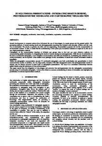
is minimized among all spatial sampling schemes S. The wi represent user-de® ned weights, and f i the realized distribution of point pairs. Figure 2 shows two di erent optimized sampling schemes according to this criterion. Figure 2 (a) consists of 16 previously sampled locations along a rectangular grid to which 14 points are added such that a uniform distribution of point pairs over the distance classes is aimed at. Figure 2 (b) consists of 30 optimally located points, without previously sampled locations, such that a uniform distribution over both direction and distance classes is aimed at and is actually obtained. C2 : even spreading of points over an area. The C2 criterion spreads the sampling points evenly over the sampling area. For ns samples it minimizes the average distance between ne random locations in the sample area and the nearest sampling points: C2 (S) =

ne j =1

min{d( pe,j , ps,i ), i = 1, ¼

, ns }

(6)

ne

where ps,i denotes the i-th sampling point, and pe,j denotes the j-th random point, with ne & ns . This criterion is especially useful in areas where grid sampling is not feasible because of complex sampling barriers or many previously sampled locations. In such situations, it can yield an improvement of up to 30 per cent. 2.7. Decision support Remotely-sensed images are often used for environmental and agricultural decision making. Although images as such may be used, commonly agricultural models play an important role, e.g., leading to various land use scenarios. A general aim is to ® nd a speci® c object O, in particular at an unvisited location. This might be a mineral vein, a location with severe pollution (or with virtually no pollution), a highly suitable soil for some crop, etc. Then for any pixel p × A we can consider the proposition `p contains an object of type O’ or `p is contained in an object of type O’. The m

(a)

(b)

Figure 2. Optimized sampling scheme for estimating an isotropic variogram with earlier measurements on a grid (a), and for an anisotropic variogram without earlier measurements (b).


1801

layers of information at every p × A can be represented in a quantitative form by {(vk ( p), k = 1, ¼ , m), p × A }. We may regard the quantization vk as a function of A into a ® nite interval for the kth layer. This approach puts several questions, which are to be solved by spatial statistics. 1. How to identify relevant objects O ? 2. How to assign any pixel p to an identi® ed object O ? 3. How to go from point measurements to values at unobserved pixels p? We consider here three possibilities: direct use of remotely sensed images, use of the utility method and ® nally use of hydrological models relying on remote sensing as an example for the use of models. (a) Direct use of remotely-sensed images is related to quantitative modeling for data integration. In this approach a relative favourability index function rk is de® ned for each layer L k as rk : [mink , maxk ] rk : [ 1, ¼

, nk ]

[0, 1] if L k is continuous [ 0, 1 ] if L k is discrete

where rk (d) × [ 0, 1 ] represents the sureness of a proposition given the evidence of d at L k . The relation fk = rk 0 vk , i.e., rk preceded by vk , de® nes the favourability of p × A to the interval [0, 1] for the kth layer L k . An fk value close to 1 corresponds to high favourability, a value close to 0 to low favourability. The favourability may have many interpretations, such as probability, a certainty, a subjective belief, a plausibility or a possibility (Chung and Fabbri 1993). ( b) When developing automated decision procedures, the user may be able to specify his objectives and preferences to the system. Then the system must be able to select the best decision. The utility method captures di erent situations in a variable C with domain {c1 , ¼ , ck }. With M possible decisions, the decision variable D has domain {d1 , ¼ , d M}. The utilities are speci® ed as u(D = di 9 C = cj ). This is for each decision D = d i computed as uÃ (D = di ) =

k j =1

u(D = d i 9 C = cj )Pr(C = cj )

(7)

The best decision is then the one with the highest utility uÃ (D = d* ). Standard maximum likelihood classi® ers calculate for each pixel the a posteriori for all classes ci . In the presence of training data they are calculated using Bayes’ rule: Pr(C = ci | x) =

P(x |C = ci )P(C = ci ) P(x)

(8)

(Strahler 1980). The class probability densities Pr(x |C = ci ) and the P(C = ci ) can be derived from the training data, whereas the unconditional feature density P(x) is usually replaced by a normalizing factor. A utility value is then de® ned to be place dependent, and relates the utility of a decision depending upon the location in the area. To model this dependence, all utility values for all possible decisions are established ® rst, and are then compensated for spatial variation in the expected utility values. Assuming that the spatial variation is multiplicative (at location x it is three times larger than at location y), GIS-based maps for each of the possible decisions can be made (Gorte and Stein, in press).

1802

A. Stein et al.

(c) Decision support may rely on application of agricultural models. Examples include crop models, soil water models and hydrological models. Many of these models require the use of remotely-sensed data: some combination with ® eld data is necessary to use optimally these data. An interesting example concerns thermal remote sensing. Meteorologists rely for short term weather forecasts and prediction of atmospheric circulation processes on correct estimation of sensible and latent heat ¯ uxes (Harding et al. 1996). Knowledge of the regional surface ¯ ux densities is thus essential in describing land surface processes in general. Di erent classes of thermal remote sensing algorithms have been identi® ed as well as evaluation of their potential applications at local and regional scale, leading to the surface energy balance for land (Bastiaanssen 1996 a). Thermal remote sensing combines ® eld measurements of the non-linear relation between surface temperature and latent heat ¯ ux. Probably thermal remote sensing can bridge the gap between ® eld measurements and grid squares used for thermal modelling by interpolating land surface processes spatially to pixels unsampled in situ and as such estimating area-representative ¯ ux densities, resistances to ¯ ow and soil water content for all pixels. 3. Practical case studies 3.1. Groundwater at di erent scales In the ® rst practical case study we investigate the use of satellite data for strati® cation of a study area to the zinc concentrations in the groundwater at di erent scales. The study area consists of the city of Oss and of a group of parcels in its vicinity in the southern Netherlands (Stein et al. 1996). We investigated whether land use as observed with remote sensing was useful as an explanatory variable at di erent scales. Concentrations of zinc [Zn] in water samples were obtained from observation wells at 2± 4 m depth: 86 wells occur within the city and 25 within the parcel group. In this study the scale is de® ned as the ratio between distance on the map and distance on the ground. Interactions between heavy metal concentrations and environmental processes occur at di erent scales. A classi® cation at the city level (® gure 3(a))was based on land use using a map in digital raster format (Thunnissen et al. 1992). The image consists of raster cells of size 25 m by 25 m. At the city level therefore a grid cell size of 25 m by 25 m was adopted. A grid cell size of 10 m by 10 m was used at the parcel level. At this level the LGN-® les were used as well, although their resolution was high as compared to the representativeness of the zinc measurements (1000 m by 1000 m). In addition, a land use map of scale 1 : 1000 produced in 1993 was used. At the city level, classi® cation yielded lower coe cients of variation (CVs) for the individual classes than for the unclassed area (table 2). Di erences are small, however, and all CVs were higher than 0´5. The mean [Zn] for built-on and greenbelt is signi® cantly higher ( p = 0´01) than for maize. At the city scale, therefore, a classi® ed TM image could be used because the basic scales match, yielding a useful classi® cation that could be used for regionalization. At the parcel level, however, the scales of the satellite image and the digitized parcels did not match (® gure 3(b)). Classi® cation with the separately constructed land use map showed high CVs of the separate land use classes as compared to that of the unclassed area. These results indicate the need for adequate scale matching. Classi® cation based on land use can be used to modify global regulations into area speci® c regulations for levels of heavy metals such as Zn in the phreatic groundwater. Arc/Info’s GRID

(a) Remote sensing image of the city of Oss.

1803

Figure 3.


Figure 3. (b) Remote sensing classi® cation (upper-left) and land use map (upper-right) to be combined with the Zn concentrations in the ground water (lower-right).

1804 A. Stein et al.

1805


Table 2. Descriptive statistics for Zn [mg lÕ 1 ] classed for land use class at the two scales. Statistically similar groups (determined by t-testing) are indicated by a and b. N

Mean

Std. Dev.

Test

CV

Min.

Max.

City scale Grass Maize Built-on Greenbelt Total

15 19 40 12 86

185´4 97´7 313´0 455´6 263´1

229´3 50´0 422´5 451´9 367

a a ab b

1´24 0´51 1´35 0´99 1´39

10´0 10´0 8´1 33´0 8´1

865 210 1650 1600 1650

Parcel scale Grass Maize Other Total

5 9 18 31

151´8 179´5 241´8 193´8

154´8 184´4 211´3 211´0

1´02 1´03 0´87 1´09

20 20 10 10

480 650 865 865

module and the ISATIS package (Geovariances 1995) allows the use of digitized maps in vector format together with maps in raster format for overlay operations. 3.2. Spatial variability in river terraces The second case study applies geostatistical procedures to a chronosequence formed by the terraces of the Henares river (approximately 40 km NE of Madrid). The terraces are clearly delineated on remotely sensed images. The aim of this study was to characterize di erences in soil properties which can be observed on clearly distinct, seemingly homogeneous geographical units. The study area is located on the southern slope of the AylloÂ n range, ranging from 600 to 900 m above sea level. Climatic ¯ uctuations, tectonic movements and lithologic-structural controls have all in¯ uenced the genesis of the river basin resulting in an assymetric valley. Actually, up to 20 topographic levels are recognized on the right bank, and a series of incised glacis-terrace ® elds at the left bank. The soils of the terraces constitute a topochronosequence that includes Entisols, Inceptisols and Al® sols. Currently, the land is mainly used for rainfed agriculture. To study soil variability within the river valley, three squared grid areas of 540 m by 540 m were sampled: one on a lower terrace (T29 ), one on a middle terrace (T25 ) and one on a higher terrace (T15 ), covering the high, middle and low Pleistocene, respectively. For each sample area, three sampling intervals of 10, 30 and 90 m with 49 observations for each distance interval were applied. Such a sampling scheme allows one to study variability at di erent scales. At each observation point, samples were taken at three depths: 0´1± 0´2 m (D1 ) , 0´4± 0´5 m (D2 ) and 0´9± 1 m (D3 ). Soil samples were analyzed for sand, silt, clay, organic carbon, calcium carbonate contents and pH (H2 O). Organic carbon was analysed at D1 in all areas and also at D2 and D3 in the lower terrace (T29 ). Table 3 shows variogram models and ranges (between brackets) for the di erent plots. All the common models have been ® tted to the soil properties of the Henares river terraces. Transitive models describe the spatial dependence for the recent terrace (T29 ), while the linear model ® ts most of the variograms of the old terrace (T15 ). The latter model indicates a still increasing variability and suggests that spatial dependence extends beyond the current sampling scheme. This re¯ ects the tendency to soil uniformization from low to high terraces.

1806

A. Stein et al.

Table 3. Summary of the best ® tting models and ranges for the three sampled areas along the Henares river. Models applied are the Spherical (Sph), Hole e ect (Hole), Gaussian (Gauss), Exponential (Exp) and pure Nugget (Nugget). Range values [m] are given in brackets. Area T29 T25 T15

Depth

Sand (%)

Silt (%)

Clay (%)

pH

D1 D2 D3 D1 D2 D1 D2 D3

Hole(27) Sph(131) Nugget Nugget Nugget Nugget Linear Linear

Gauss(66) Sph(84) Nugget Hole(26) Linear Linear Linear Linear

Sph(76) Exp(71) Nugget Nugget Nugget Linear Linear Linear

Hole(27) Gauss(55) Nugget Sph(161) Exp(50) Sph(100) Linear Unde® ned

CaCO3 (mg kgÕ 1 )

OC (mg)

Ð

Sph(65) Hole(23) Nugget

Sph(93) Nugget Nugget Linear

Ð

Linear

Ð

Ð Unde® ned Linear

Ð Ð

At D3 in T29 all variables exhibit a pure nugget e ect, indicating absence of spatial dependence. It arises from large point-to-point variation at short distances, caused by irregularities of the underlying gravel layer. In that case, an increase in the detail of sampling is required to reveal the spatial structure of soil properties. Spatial variability modelled with variograms in the study area shows that all standard models are applicable to the area. A larger variety of models describes the properties of the low (recent) terrace (T29 ) whereas the linear model ® ts most of the variograms of properties of the high (old) terrace (T15 ). Therefore, ageing of the terraces causes the variables to show non-transitive variogram models. We conclude from this study that the variability of the soil properties decreases from younger to older deposits as soils tend to increasing uniformization as a function of age. 3.3. Classi® cation with the indicator kriging classi® er Classi® ction with the indicator kriging classi® er (see § 2.4) was tested two-fold: ® rst using spatial simulations, and second using actual data. First, 2000 pixel spectra were characterized in three image bands to represent a mineral with a ® ctive absorption feature: two bands on the absorption shoulder and one in the centre of the absorption feature. These pixels are used as conditioning data set for a sequential Gaussian simulation (Journel and Alabert 1989, Deutsch and Journel 1992 to create three spectral image bands. From the resulting image bands, 1000 of the pixels known to exhibit the absorption feature are used to train the classi® ers and 1000 image pixels from the conditioning data set are used to assess the accuracy of the classi® ers. For images with low nugget variance or small additive noise levels the indicator kriging classi® er clearly yields the best results (® gure 4). With increasing nugget variance the classi® cation accuracy decreases for the indicator kriging classi® er while the supervised classi® cation techniques remains constant despite a ¯ uctuation of 10 per cent around a mean value of accuracy. When the noise level exceeds approximately 25 per cent of the total variance, the classi® cation accuracy for the indicator kriging classi® er has decreased to a similar value as found for the k-nearest neighbour classi® er. When the nugget variance equals 50 per cent of the total variance, the indicator kriging classi® er becomes less accurate than the parallelepiped classi® er, being the least reliable supervised classi® cation technique. To test the performance of the indicator kriging based method for feature extraction on real data, we used a small area from the Cuprite Airborne Visible


1807

Figure 4. Estimates of accuracy of the indicator kriging classi® er with changing nugget e ect as a percentage of the sill value (* : indicator classi® er, D : k-nearest neighbour, +: parallelepiped, E : maximum likelihood).

Infrared Image Spectrometer (AVIRIS) data set. The area is 50 by 20 pixels in size and contains both kaolinite and alunite outcrops. Three bands were used to characterize the mineral absorption features of both kaolinite and alunite in the 2´10± 2´20 mm wavelength range. When comparing known occurrences of kaolinite and alunite with predicted occurrences the indicator approach proved to be more reliable than standard classi® cation techniques. A further improvement to sub-pixel analysis as described below is shown in ® gure 5. Here we give probability maps for undivided mineral abundance nested in a three-dimensional data cube. The sides are colour coded sliced images for the top and right-hand column of the image in which each slice represents one mineral. The summation of these at a pixel yields the total 100 per cent area of the pixel. Thus the probabilities are interpreted as an areal percentage at each mineral phase. 3.4. Fuzzy classi® cation of landscape units in southern Spain Fuzzy classi® cation of landscape units was implemented on data from a 20 ha study site located near the village Alora in southern Spain. A DEM with 5 m resolution was created through interpolation of elevation data obtained via image matching of scanned aerial photographs. The interpolation was performed using ARC/INFO’s procedure TOPOGRID. The topographic attributes used in the clustering procedure were: elevation, slope, plan curvature, pro® le curvature, stream power index and wetness index, also referred to as the compound topographic index. The cluster analysis involved 8412 grid cells. To represent a soil-landscape model the fuzzy c-means clustering of attribute data describing surface topography was applied. To judge the validity of the fuzzy partition its predictive power was evaluated on an independently measured soil property. This approach is di erent from the validity functionals, entirely based on information obtained from within the clustering process (Bezdek 1981, Roubens 1982). It was investigated to which degree a fuzzy

1808

A. Stein et al.

Figure 5. Three-dimensional datacube where the two-dimensional slices show mineral maps for 15 di erent minerals derived from indicator probability classi® cation using AVIRIS data from Cuprite.

c-means clustering of attribute data derived from a DEM can reveal spatial clusters

that closely resemble the soil-landscape units. This approach enhances the conventional soil-landscape modelling methodology because it allows representation of the fuzziness inherent to soil-landscape units. For any speci® ed number c of clusters less than the number of data (2 < c < n) and every fuzziness exponent, (w> 1) the fuzzy c-means algorithm will produce clusters. Least-squares linear regression analysis was applied to relate top soil clay data to cluster membership values obtained with di erent combinations of c and w 2 using 38 sample points. R values are plotted in ® gure 6. The optimal fuzzy partition, obtained when the largest proportion of the variation in clay content is explained 2 by the model, occurs at c = 4 and w= 2.1, with R = 0´73. The use of more clusters 2 does not further increase R . Fuzzy c-means classi® cation of attribute data derived from a DEM reveals spatial clusters that closely resemble soil-landscape units. The use of a least-squares regression for cluster validity evaluation requires further attention involving also other classi® cation methods, in particular those using prior knowledge. 3.5. Pixel resolutions and scales in thermography and implications for evaporation mapping Longwave spectral measurements are through Planck’s law and after applying atmospheric corrections related to the temperature of the land surface. Spaceborne thermal infrared scanners can thus be used to retrieve the land surface temperature on a pixel-by-pixel basis. The land surface temperature reveals the thermodynamic equilibrium between the incoming short and longwave radiation and the hydrological


1809

Figure 6. R 2-values of the linear relation between top soil clay content and fuzzy cluster membership values for di erent values of c and f .

status of the land surface, i.e., the partitioning between net radiation into sensible and latent heat ¯ uxes. Wet and vegetated surface elements are cooled by evaporation whereas dry and bare soils are usually heated by solar radiation resulting in a signi® cant higher equilibrium surface temperature. Pixel wise information on surface temperature can be converted into evaporation ¯ uxes. This information is important at various scales: evaporation at ® eld scale is bene® cial to determine crop stress and to allow precision farming (pixels ~100 m, Thematic Mapper, e.g., Bastiaanssen et al., 1996 b). Watershed management is related to regional water balances and demands evaporation to be speci® ed at a much coarser scale; the pixels can therefore be much larger (pixels ~1 km, NOAA-AVHRR). Atmospheric studies for weather and climate prediction need information on land surface heat ¯ uxes at a horizontal scale of thousands of kilometres being typically covered by Meteosat thermal images (Hurk et al., 1997). This indicates the need for a wide range of pixel resolutions and spatial scales for thermal images. Geostatistics can help to select the best pixel size. Conversion of surface temperature to heat ¯ uxes has some constraints with respect to pixel resolution and scale: 1. The relation between surface temperature and ¯ uxes is non-linear at a horizontal scale of several hundreds of metres. Hence application of large NOAAAVHRR and Meteosat pixels in heterogeneous landscapes with a large sill level can lead to erroneous results. Therefore, the sill level needs to be determined. 2. The relation between surface temperature and ¯ uxes depends upon radiation levels, surface albedo and vegetation index. Therefore a complex transformation algorithm is required; 3. Land surface processes have a microscale character. For example, temperature of leaves di ers from temperature of bare soil portions. This is not captured when

1810

A. Stein et al.

the pixel size is much larger than the length scale of the processes. Hence, the range needs to be determined. The Surface Energy Balance Algorithm for Land (SEBAL) has been designed to meet these constraints as much as possible. Heat ¯ uxes are parameterized to behave as pixel dependent heat and water vapour sources. For each pixel corrections are made for net absorbed radiation (albedo) and vegetation e ects (vegetation index). The natural character of the scale dependent non-linear relationship between surface temperature and heat ¯ uxes changes with the landscape and statistical procedures can be applied to express the scale dependency between land surface elements. The resolution and scale treatments can be understood by studying evaporation variograms. Figure 7 shows the variogram of evaporative fraction, i.e. the evaporation normalized for absorbed radiation, using airborne 20 m pixel resolution thermal data to calculate heat ¯ uxes (Bastiaanssen et al. 1996 c). The range of the variogram is approximately 3000 m and much spatial variation is present among land surface elements smaller than 400 m. Hence a location dependent description of the sensible and heat ¯ uxes can only be made with a pixel resolution below 400 m. Therefore, Landsat Thematic Mapper images should be taken. The e ect of shifting from Thematic Mapper images to NOAA-AVHRR images is shown in ® gure 8. Precise information on ® eld scale conditions cannot be detected and the larger pixels show a mixture of land surface conditions with unnatural sharp boundaries between pixels. For a pixel size of 5 km, a homogeneous evaporation map can be expected (® gure 7), whereas ® gure 8 shows that the average of 25 pixels will yield an even evaporation pattern. Hence, the NOAA-AVHRR pixel size is suitable to detect evaporation on the water balance of a watershed of approximately 20 km by 20 km and Meteosat should be selected for thermal studies at (sub-) national scale. 4. Discussion: what’s in a pixel? From the above case studies the pixel values emerge as a number which ® lls a two-dimensional plane surface as a scale reduction representing the ground. Although

Figure 7. Variogram of evaporative fraction (latent heat ¯ ux/net available energy) for a transect in an irrigated Mediterranean landscape, Castilla la Mancha, Spain.

Figure 8.

Map of actual evaporation in Aggulart de la Frontera, Cordoba Province (Spain), 2 July, 1990. E ects of shift in pixel size are demonstrated. (a) Landsat TM, (b) aggregation to NOAA pixel size.


1811

1812

A. Stein et al.

a straightforward relation is likely to exist, much uncertainty, and hence much potential use of statistical procedures, is still present. The basic problem is that a pixel, or the related instantaneous ® eld of view on the ground (IFOV), is often larger than required. The pixel size is important because a sensor seemingly receives all the radiation from the IFOV and generates a response proportional to the quantity of radiation received. Several problems arise: continuous movement within the instrument, or of the spacecraft; non-uniform response of the scanner to radiation from within the IFOV as well as response to radiation from outside the IFOV; pixel intensities are correlated. Recent research has focused on the optical point spread function to describe the intensity as a function of position in the focal plane arising from an object which is a point source with its geometrical image being a point in the focal plane. The point spread function is of practical importance for (i ) objects that are very small in relation to the IFOV, (ii) mixed pixels, and (iii ) o -nadir viewing of the ground. For example, mixed pixels occur where structure on a small scale, relative to the IFOV, exists, for example gas ¯ ares, blast furnaces and agricultural straw ® res. When creating an image it is common to use a grid in a regular network of geographical coordinates. Interpolation methods of image intensity values at such a grid from the navigated grid (resampling) include nearest neighbour methods and bilinear and bicubic interpolation. The choice of which to use depends upon the use to which the data will be put and upon the computer facilities that are available. For classi® cation, however, use of interpolated data may have an adverse e ect because of smoothing. It may, therefore, be decided to classify the raw data ® rst, followed by geometrical recti® cation. The standard deviation of a geometrical recti® cation can be around 80± 90 per cent of the length of the edge of the IFOV. To achieve a better accuracy, a recently developed method uses digitized small extracts (or chips) from higher resolution data (Cracknell and Paithoonwattanakij 1989). The geometrical recti® cation has an error equal to a fraction of the lineardimensions of the IFOV with the AVHRR data. It may be as low as only 20 per cent of the edge of the IFOV. 5. Conclusions This paper shows that an integrated approach towards spatial statistics for remote sensing is possible and necessary. Each of the topics distinguished above (scale, classi® cation, sampling and decision support) relies on a quantitative, spatial approach. Hence, spatial statistical procedures, with their emphasis on the relation between quantitative satellite images and the position in the ® eld can be used. A basic distinction concerns the layers of information, being either quantitative or qualitative. It was shown in this study how it could be used to combine data collected at di erent scales, either by spatial interpolation or by classi® cation. It was shown how modern sampling procedures can be developed which take existing soil boundaries into account. Use of satellite images for decision support ® nally introduces the concept of the spatial utility function, which integrates the di erent spatial statistical procedures. Acknowledgments The authors are grateful to the ITC for providing the means and facilities to organize this seminar. The layer concept summarized in this paper is due to the ideas of C. F. Chung, to whom we are very grateful.


1813

References Bastiaanssen, W. G. M., Menenti, M., Dolman, A. J., Feddes, R. A., and Pelgrum, H., 1996, Remote sensing parameterization of meso-scale land surface evaporation. In Radiation and Water in the Climate System, Remote Measurements, NATO-ASI Series I, Global Environmental Changes 45, edited by E. Raschke (Berlin: Springer), pp. 5401± 427. Bastiaanssen, W. G. M., Van der Wal, T., and Visser T. N. M., 1996 b, Diagnosis of regional evaporation by remote sensing to support irrigation performance assessment. Irrigation and Drainage Systems, 10, 1± 23. Bastiaanssen, W. G. M., Pelgrum, H., Menenti, M., and Feddes, R. A., 1996 c, Estimation of surface resistance and Priestley-Taylor a-parameter at di erent scales. In Scaling up in hydrology using remote sensing, edited by J. B. Stewart, E. T. Engman and R. A. Feddes (Chichester: Wiley), pp. 93± 111. Bezdek, J. C., 1981, Pattern Recognition with Fuzzy Objective Function Algorithms (New York: Plenum Press). Burrough, P. A., 1996. Natural objects with indeterminate boundaries. In Geographic Objects with Indeterminate Boundaries edited by P. A. Burrough and A. U. Frank (London: Taylor & Francis), pp. 3± 28. Chung, C. F., and Fabbri, A. G., 1993, Representation of geoscience data for information integration. Non-Renewable Resources, 2, 122± 139. Cracknell, A. P., and Paithoonwattanakij, K., 1989, Pixel and sub-pixel accuracy in geometrical recti® cation of AVHRR imagery. International Journal of Remote Sensing, 10, 661± 667. Cressie, N. A. C., 1991. Statistics for spatial data (New York: John Wiley and Sons). Curran, P., 1988, The semivariogram in remote sensing: an introduction. Remote Sensing of Environment, 24, 493± 507. De Bruin, S., and Stein, A., 1998, Soil-landscape modelling using fuzzy c-means clustering of attribute data derived from a DEM. Geoderma (in press). De Jong, S. M., and Burrough, P. A., 1995, Classi® cation of mediterranean vegetation types in remotely sensed images. Photogrammetric Engineering & Remote Sensing, 61, 1041± 1053. Deutsch, C. V., and Journel, A. G., 1992, GS-L IBÐ Geostatistical software library and user’s guide (Oxford: Oxford University Press). Gessler, P. E., Moore, A. W., McKenzie, N. J., and Ryan, P. J., 1995, Soil-landscape modelling and spatial prediction of soil attributes. International Journal of Geographical Information Systems, 9, 421± 432. Geovariances, 1995, ISAT IS (Avon: Geovariances). Gorte, B. G. H., and Stein, A., 1998, Bayesian classi® cation and class area estimation of satellite images using strati® cation. IGARS (in press). Harding, R. J., Taylor, C. M., and Finch, J. W., 1996, Areal average surface ¯ uxes from mesoscale meteorological models: the application of remote sensing. In Scaling up in Hydrology using Remote Sensing, edited by J. B. Stewart, E. T. Engman and R. A. Feddes (Chichester: Wiley), pp. 59± 76. Hole, F. D., and Campbell, J. B., 1985, Soil L andscape Analysis (London: Routledge & Kegan Paul). Hudson, B. D., 1992, The soil survey as paradigm-based science. Soil Science Society of America Journal, 56, 836± 841. Hurk, B. J. J. M., Bastiaanssen, W. G. M., Pelgrum, H., and Van den Meygaard, E., A simple procedure for assimilation of initial soil moisture ® elds in weather prediction models using METEOSAT and NOAA data. Journal of Applied Meteorology (in press). Jenny, H., 1941, Factors of Soil FormationÐ a System of Quantitative Pedology (New York: McGraw-Hill). Journel, A. G., 1983, Nonparametric estimation of spatial distributions. Mathematical Geology, 17, 445± 468. Journel, A. G., and Alabert, F., 1989, Non-Gaussian data expansion in the earth science. T erra Nova, 1, 123± 134. Journel, A. G., and Huijbregts, Chr. J., 1978, Mining Geostatistics (New York: Academic Press).

1814


Lagacherie, P., Andrieux, P., and Bouzigues, R., 1996, Fuzziness and uncertainty of soil boundaries: from reality to coding in GIS. In Geographic Objects with Indeterminate Boundaries edited by P. A. Burrough and A. U. Frank (London: Taylor & Francis), pp. 275± 286. Moore, I. D., Grayson, R. B., and Ladson, A. R., 1991, Digital terrain modelling: a review of hydrological, geomorphological, and biological applications. Hydrological Processes, 5, 3± 30. Moore, I. D., Gessler, P. E., Nielsen, G. A., and Petersen, G. A., 1993, Soil attribute prediction using terrain analysis. Soil Science Society of America Journal, 57, 443± 452. Quinn, P. F., Beven, K. J., and Lamb, R., 1995, The ln(a/tan b ) index: how to calculate it and how to use it within the TOPMODEL framework. Hydrological Processes, 9, 161± 182. Richards, J. A., 1993, Remote Sensing Digital Image Analysis: An introduction, Second Edition (Berlin: Springer-Verlag). Roubens, M., 1982, Fuzzy clustering algorithms and their cluster validity. European Journal of Operational Research, 10, 294± 301. Stein, A., Staritsky, I., Bouma, J., and Van Groenigen, J. W., 1995, Interactive GIS for environmental risk assessment. International Journal of Geographical Information Systems, 5, 509± 525. Stein, A., Varekamp, C., Van Egmond, C., and Van Zoest, R., 1996, Zinc concentrations in groundwater at di erent scales. Journal of Environmental Quality, 24, 1205± 1214. Strahler, A. H., 1980, The use of prior probabilities in maximum likelihood classi® cation of remotely sensed data. Remote Sensing of Environment, 10, 135± 163. Thunnissen, H., Olthof, R., and Getz, P., 1992. L and Use Database of the Netherlands Compiled with L andsat T hematic Mapper Data (In Dutch) (Wageningen: The Winand Staring Centre). Van der Meer, F., 1994, Extraction of mineral absorption features from high-spectral resolution data using non-parametric geostatistical techniques. International Journal of Remote Sensing, 15, 2193± 2214. Van der Meer, F., 1996, Performance of the indicator classi® er on simulated image data. International Journal of Remote Sensing, 17, 621± 627. Van Groenigen, J. W., and Stein, A., 1998, Spatial simulated annealing for designing spatial sampling schemes. Journal of Environmental Quality (in press). Van Groenigen, J. W., Stein, A., and Zuurbier, R., 1997, Optimization of environmental sampling using interactive GIS. Soil T echnology, 10, 83± 98. Warrick, A. W., and Myers, D. E., 1987, Optimization of sampling locations for variogram calculations. Water Resources Research, 3, 496± 500. Webster, R., 1985, Quantitative spatial analysis of soil in the ® eld. In Advances in Soil Science, Vol. 3, edited by B. A. Stewart (New York: Springer-Verlag), pp. 1± 70. Wilding, L. P., and Drees, L. R., 1983, Spatial variability andpedology. In Pedogenesis and Soil T axonomy. I. Concepts and interactions, edited by L. P. Wilding, N. E. Smeck and G. F. Hall (Amsterdam: Elsevier), pp. 83± 116. Zadeh, L. A., 1965, Fuzzy sets. Information and Control, 8, 338± 353.