Integrating tracer with remote sensing techniques for

Integrated Methods in Catchment Hydrology—Tracer, Remote Sensing and New Hydrometric Techniques (Proceedings o f IUGG 99 Symposium HS4, Birmingham, July 1999). IAHS Publ. no. 258, 1999.

75

Integrating tracer with remote sensing techniques for determining dispersion coefficients of the Dâmbovita River, Romania

MARY-JEANNE ADLER, GEORGE STANCALIE & CRISTINA RADUCU National Institute of Meteorology and Hydrology, Sos Bucuresti-Ploiesti Romania e-mail: [email protected]

97, 71552

Bucharest,

Abstract Knowledge of dispersion coefficients in longitudinal, lateral and vertical flow directions is of utmost importance when evaluating the timeconcentration distribution of pollutants at any point in a stream. Remotely sensed field data (from the National Administration of the Ocean and Atmosphere and télédétection) were used to identify the river sector for a dye tracing experiment. The main criteria were to locate a sector without significant anthropogenic influence and with similar hydraulic conditions. The sector selected for sampling was 2.5 km long. The longitudinal and threedimensional dispersion coefficients were determined. The time-concentration curve for rhodamine dye obtained under different hydraulic conditions of flow (different stages) was measured on the Dâmbovita River. The stage was nearly constant for each experiment but different in each case, therefore it was possible to obtain information for different regimes. Additional information needed to make use of the one-dimensional and three-dimensional mathematical models of dispersion was obtained at the Malu cu Flori gauging station (continuos stage recording and stage-discharge curve). Finally, the experimental data were used to verify the mathematical dispersion model proposed for the Dâmbovita River.

INTRODUCTION Stream dispersion phenomena, dilution and transport of pollutants in a channel is caused by advective and diffusive transport mechanisms. The range of the dispersion coefficients in the longitudinal, lateral and vertical directions of flow is very important in evaluating the time-concentration distribution of a pollutant at any point in a stream. Although significant advances have been made in understanding and modelling dispersion in natural streams, the problem of dispersion coefficients based on field and experimental data needs further study. The main aim of the experiment was to determine the dispersion coefficients and to verify the predicted concentration by the proposed mathematical model. The remotely sensed data from the National Administration of the Ocean and Atmosphere were useful in identifying the river sector. However the spatial resolution used for dispersion was inadequate for mapping the river. Additional télédétection data had also to be used. In the first section of the paper, the dispersion model is presented; in the second, both the experiment and the resulting data are shown.

76

Mary-Jeanne

Adler et al.

MATHEMATICAL MODEL OF DISPERSION The concentration distribution of a dye in a turbulent stream is governed by an equation based on the law of conservation of mass (Landau & Lifchitz, 1971). In the case of no other sinks and sources in the reach that is:

- dc dt d xi d xi - + Vi

D

i

J

dc , _D dc ~

- -

(1)

+

c is the mean local concentration of dye (parts per billion by volume), v is the mean velocity (/ refers to Cartesian coordinates x, y, z considered in the direction of flow, transversal, along it and vertically down, respectively), Dy and D are the turbulent and molecular diffusion coefficients; v is the longitudinal velocity. The diffusion and convective terms are neglected due to the mean velocity components in the y and z directions (because they are usually small compared with the v term). Considering A = (D , D , D ), equation (1) becomes: x

x

x

y

z

2

dc - dc _ d c + V;

&

=

(2)

D

d 'dxjdxi Xi

The initial condition is:

(3)

c(x, y, z) - 0 for x > 0, y > 0 and z > 0 The boundary conditions are: c(x, y, z,t) = 0 for all values of t

dc

dc

--» 0 as x —> °=; >0 as y —> °= (physicallyy = 5/2) —» 0 as z —» oc (physically z = H)

dz dx

Assuming D -D could be written: x

dy

and mean velocity v - V for the reach, the solution of equation (2) x

M

c(x,y,z,t) =

(x~Vtf

exp

ADt

exp

jAnDt

y AD t y

•yJAllDj

exp

ADt

(4)

which does not satisfy the first boundary condition, but:

\~ T \°° c(x,y,z,t)àxâyàz = M

(5)

J—oo J—oo J—CO

To support the physical meaning of the river, this can be approximated as:

jJI

c(x,y,z,t)dxdydz = M -

- |_ j_ c(x, y, z, t)éxàyàz M

j

^

J_^ c(x, y, z, r)dxdydz - j^ _j'^ \ jc(x, y, z,

(6) which indicates that for natural flow conditions in a stream, with finite values of B (the

Integrating

tracer with remote sensing

techniques

for determining

dispersion

coefficients

11

surface width) and H (the depth of flow), the amount of dye recovered would be less than the total amount of dye injected. The amount of dye lost or detained in dead zones laterally and vertically is assumed to be given by the three quantities on the right-hand side of the equation. Equation (3) is valid for a short interval of time because it does not take into account the amount of dye that may be lost due to absorption and decay. For downstream distances far from the injection point, equation (3) may be necessary to account for such a loss. Equation (3), known as the three-dimensional mathematical model of dispersion, has been used to determine the vertical and lateral dispersion coeffi­ cients for different reaches of the stream where the measured time-concentration curves of dye are available. The value of D is assumed to be equal to the value of longitudinal dispersion D, determined from the one-dimensional mathematical model of dispersion. Assuming that mixing is uniform at the measurement cross-section, the onedimensional case with a constant longitudinal dispersion coefficient (D„ = D), the equation for the mean concentration obtained from equation (1) following the standard procedure of averaging is: x

2

de - dc dc -—+ v, =D

._. (7)

where v = V is the average velocity of flow at a section which is assumed to be independent of time. ;

{x-Vtf / s (8) c(x, t) = — , exp 4Dt A^AtzDt It may be observed that D may not be the same as D, but for larger values of either x or t, D = D. The lateral dispersion coefficient D is expected to depend on the vertical dispersion coefficient D ; of B, H, and V and the mean velocity of flow at the sampling station, V . A dimensional analysis shows that (Bansal, 1981): M

1

x

X

y

z

s

~}M '

V

l

(9)

J 3

1

in which V = QIA, V = x/t and Q is the discharge (m s" ); A is the area of the crosssection (m ); x is the distance from the point of injection (m); and t is the travel time (h). D is determined from the best fit between the computed and the measured timeconcentration curves. For a value of D the concentration distribution can be computed from the three-dimensional mathematical model of dispersion. s

p

2

p

z

z

Adaptation of the mathematical model of dispersion to the river conditions The loss of solute concentration increases downstream as the distance x increases. Using the linearity of the problem, a modified solution of equation (7) first suggested is: c(x,t)-

M Vt Asl4%Dt

I exp

2

(x-Vt) ' ADt

(10)

78

Mary-Jeanne

Adler et al.

which appears to take the dye loss into account, as the term is linear of x. But in natural streams an amount of dye is lost due to photochemical decay and benthic adsorption by vegetation and suspended solids present in the stream, as well as by retention in the dead areas. So (10) is adjusted to take this into account, giving: /

\-K

n

~K

0

ix-Vtf ADt

M exp A^AnDt

1

x

Vt

(11)

in which K is a regional dispersion factor defined for a stream and Ko is a coefficient of loss of dye in a reach. K was determined by trial and error by comparing the computed and observed time-concentration curves for the stream and Ko was derived from a dimensional analysis of the dependent factors: VB 4D

logjlHIL) \og(Dt /L )

|

2

y

p

K

(12)

1 j

VBIAD is a loss factor accounting for the detention of dye in lateral dead zones; log(2H/L)/log(Dt /L ) is a loss factor accounting for the detention of dye in the vertical dead zones; K\ ~ 0.5 accounts for the loss of dye due to decay and adsorption which is relatively constant in streams. Finally, the one-dimensional mathematical model of dispersion in a stream can be described by: 2

p

/

^

c(x,t) =

1

1-

xB \6Dt

x

\og(2HIL) AVt\og(Dt IL ) 2

2

M ^exp

(x-Vt) ADt

(13)

a4aHd\ K This is a linear solution of equation (7) that satisfies all the necessary initial and boundary conditions required in the case of a natural stream. The value of D, which p

Altitude (m) 2300 2200 2100

VBÊSL

-

2000 1900

1

1800

— j

-' 1 7 0 0

WÊÊÊ

1600 -•1500 •'•',1400 1300

,j

H '•

1200

I0 -M000 900

111

r - l 800 !

1700

i—1600 -—^500

Fig. 1 The numerical model of the Dâmbovita River basin.

Integrating

tracer with remote sensing

techniques

for determining

dispersion

coefficients

79

gives the best fit between the computed and measured time-concentration curves, is accepted as an appropriate value for the reach.

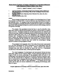
EXPERIMENTAL DATA Using a local image of the basin, a 2.5 Ion section of the Dâmbovita River was chosen for the experiment. The digital elevation model of the river basin is presented in Fig. 1. The additional information needed to make use of the one-dimensional and threedimensional mathematical models of dispersion was obtained at the Malu cu Flori gauging station on the Dâmbovita River. We conducted tracer experiments on the Dâmbovita River in 1995 (Q = 12.9 m s" ) and 1997 (Q = 7.88 m s" ). Rhodamine B dye was injected instantane­ ously into the river. Concentration distributions were measured at four cross-sections downstream from the point of injection. The concentrations for each section were measured using a fluorometer. Gaspar & Oreaeanu (1987) presented the method. Incomplete mixing over the width of the river is very important. Therefore all samples were taken simultaneously at three sites at each cross section of the river. In the last control section full mixing was assumed and dye concentrations were measured using a single fluorometer. The dispersion coefficients were directly proportional to the breakthrough. Greater dispersion coefficients were reflected by decreased peak breakthrough concentrations as the tracer migrated downstream (Figs 2 and 3). 3

1

3

2 0 0

1

Ti n e C s e c u n d )

~*

Fig. 2 Tracer-response curve for stream sections in 1995.

"

~

~ *

2O00

80

Mary-Jeanne

Adler et al.

0.35

time (min) Fig. 3 Tracer-response curve for stream sections in 1997.

VERIFICATION OF THE MATHEMATICAL DISPERSION MODEL To verify the correctness of the longitudinal dispersion coefficient as predicted from the one-dimensional model, a test was required to check the response of the model at different locations along the stream (Fig. 4). The computed curve is obtained by determining D, K, and Ki in the first section of the experiment; these values are used to calculate the peak concentration by equation (13). Figure 4 shows that the deviation is not significant and the check proves that the one-dimensional model of dispersion functioned satisfactorily.

Integrating

tracer with remote sensing

techniques

for determining

dispersion

coefficients

81

The experiment allowed us to have some idea of the degree of magnitude of the coefficients of dispersion. In the Malu cu Flori gauging station section, the values obtained were: D = D - 20 m s" , for Q = 12.9 m V (K = 0.40 and K\ = 0) and D = D = 11.5 m s" , D = 0.085 m s" , D = 0.000 06 m s" for Q = 7.88 m s" (K = 0.27, * i = 0). The results of the three-dimensional model of dispersion for the 1997 experiment, which permitted us to identify all the components of the dispersion vector for one section, are shown in Fig. 5. 2

1

2

1

1

x

2

x

1

y

2

1

3

1

z

Fig. 5 Three-dimensional dispersion model of the Dâmbovita River.

CONCLUSION The predicted values of D agree well with the dispersion characteristics of the stream. The values are dependent on the flow regime of the river. In conclusion, one experiment is not sufficient to determine the coefficient of dispersion, but a relationship depending of the river regime and the hydraulic conditions of flow has to be obtained.

REFERENCES Bansal, M. K. (1981) Dispersion in natural streams. J. Hydraul. Div. ASCE 97(HY11), 95-110. Gaspar, E. & Oraseanu, I. (1987) Natural and artificial tracers in the study of the hydrodynamics of karst. Theorel. Appt. Karstology 3. Landau, L. & Lifchitz, E. (1971) Mécanique des Fluides. Edition MIR, Moscow.

Integrated Methods in Catchment Hydrology—Tracer, Remote Sensing and New Hydrometric Techniques (Proceedings o f l U G G 99 Symposium HS4, Birmingham, July 1999). IAHS Publ. no. 258, 1999.

83

Application de la thermogaphie infrarouge aéroportée à l'étude de l'hétérogénéité d'une zone humide riveraine d'un cours d'eau

CELINE PINET, HOCINE BENDJOUDI Laboratoire de Géologie Appliquée, F-75252 Paris, France

Université Pierre et Marie Curie, 4 Place

Jussieu,

e-mail: [email protected]

ROGER GUERIN Département de Géophysique Appliquée, Université Pierre et Marie Curie, Paris,

France

Résumé La compréhension du fonctionnement des zones humides riveraines du cours moyen des rivières passe par la reconstitution et la modélisation de la mise en place des alluvions qui leur servent de substrat. Sur les zones humides des vallées de l'Aube et de la Seine, une prospection thermique aéroportée a ainsi été mise en œuvre, dans le but de fournir des images dans le visible et le thermique lointain. Suite aux premiers résultats obtenus—distinction entre les zones d'eau libre et les zones d'eau stagnantes, localisation rapide et à grande échelle des anciens réseaux hydrographiques—un site test d'une superficie de 1 ha a été sélectionné sur un des axes de vol. Les mesures électromagnétiques et les sondages réalisés sur ce site ont révélés une concordance des résultats sur les sols vierges de toute pratique agricole. D'autres investigations géophysiques mais également géochimiques (traceurs), permettraient à l'avenir de définir les paramètres hydrauliques de cette zone humide.

INTRODUCTION La prise de conscience de l'importance des différentes fonctions jouées par les zones humides, fonctions écologiques (productivité primaire, habitat pour de nombreuses espèces ...) mais également hydrologiques (régulation des régimes hydrologiques, épuration physique et chimique de l'eau ...) ainsi que la disparition ou la dégradation de 50 à 60% de ces milieux dans la plupart des pays (Fustec et al, 1996), ont conduit le gouvernement français à adopter, en 1995, un plan national d'action pour les zones humides. Parmi les axes de ce plan, le Programme National de Recherche sur les Zones Humides (PNRZH), lancé en janvier 1997, propose l'étude de plusieurs sites représentatifs—zones humides alluviales, littorales et intérieures—permettant de définir de nouvelles méthodes de gestion et de conservation de ces milieux.

PROGRAMME DE RECHERCHE Dans le cadre du PNRZH, le Laboratoire de Géologie Appliquée de l'Université Pierre et Marie Curie (France) développe une approche interdisciplinaire et originale, basée sur la mise au point d'outils d'investigation sur le thème "Fonctionnement des zones

84

Celine Pinet et al.

humides riveraines du cours moyen des rivières: analyse et modélisation de la genèse des hétérogénéités structurales et fonctionnelles, application à la Seine moyenne". Ce projet de recherche s'articule en trois grandes parties—-analyse du remplissage sédimentaire, étude du fonctionnement hydrique du système et étude des flux et bilans de matière—qui devront permettre d'aboutir à une typologie opérationnelle à même d'éclairer les décisions de gestion. A ces trois volets s'ajoute l'étude des impacts anthropiques à l'échelle historique (de la période médiévale jusqu'aux années 3 0 ^ 0 ) et au cours des cinquante dernières années, durant lesquelles le rythme des actions d'aménagement s'est accéléré.

SITE D'ETUDE

Le site choisi pour mettre en œuvre ce programme de recherche est la "zone atelier Seine amont". Situé au sud-est de l'agglomération parisienne, il recouvre les corridors de l'Aube et de la Seine à l'amont de leur confluence et les plaines de Romilly et de la Bassée en amont de la confluence avec l'Yonne. Cette zone a déjà été classée Zone Humide d'Importance Majeure par le Ministère français de l'Environnement.

METHODOLOGIE

Partant du principe que le fonctionnement d'une zone humide est très fortement lié à la nature et à la distribution spatiale des sédiments sous-jacents ainsi qu'à la façon dont ces matériaux se sont mis en place au cours du temps, un des axes de recherche concerne la reconstitution et la modélisation de la mise en place des alluvions qui lui servent de substrat. L'analyse de la répartition spatiale des hétérogénéités des matériaux de surface et de subsurface est ainsi nécessaire. Dans cette optique, une prospection thermique aéroportée a été effectuée en février 1997 sur sol nu, en période d'inondation, sur les vallées de la Seine et de l'Aube (Pinet, 1997). Cette méthode, déjà largement utilisée en archéologie et en pédologie (Scollar et al, 1990), a l'avantage de couvrir de grandes distances en des temps relativement brefs comparés aux méthodes d'investigation géophysique au sol.

PROSPECTION T H E R M I Q U E ET PROBLEMATIQUE

Principe La thermographie infrarouge aéroportée est basée sur la propriété qu'ont les corps d'émettre de l'énergie sous forme d'ondes électromagnétiques, qui sont enregistrées par le détecteur d'un radiomètre à balayage embarqué à bord d'un avion. Les fenêtres de transmission de l'atmosphère se situent dans les bandes de longueur d'onde 0.3-1 um et 10-13 pm, qui comprennent les domaines spectraux émis par le sol (respectivement visible et thermique). Le capteur utilisé, sensible à ces longueurs

Thermogaphie

infrarouge

aéroportée

pour l'étude

de l'hétérogénéité

d'une zone

humide

85

d'onde, permet l'acquisition d'images à la fois dans le domaine du visible et du thermique. L'émission du sol, définie par remittance W, est proportionnelle à la puissance quatrième de sa température: W = eoT

4

( n

où e, a, T sont respectivement l'émissivité du sol, la constante de Stéfan-Boltzmann et la température du sol; avec e ~ 1 et a = 5.6693 x 10" W m" K" . La température de surface du sol dépend du bilan énergétique au niveau du sol— identique en tout point de la plaine alluviale—et des processus de transfert de chaleur (par conduction et convection thermique) au sein du sol. Parmi les grandeurs caractéristiques de conduction thermique, l'inertie thermique P intègre le facteur temps dans l'étude de la réaction d'un sol face à un apport de chaleur: 8

2

4

(2) où k et C sont respectivement la conductivité thermique et la capacité calorifique. Face à un apport de chaleur, les corps conductifs ont une réponse thermique inversement proportionnelle à P. v

L'eau possédant une inertie thermique très élevée, les contrastes d'émission du sol, liés aux contrastes de température apparente du sol, sont interprétés comme des contrastes d'inertie thermique, qui sont eux-mêmes dus à la présence d'eau dans le sol.

Premiers résultats, premières questions La mission aéroportée a permis l'analyse de onze axes (d'environ 7 km de long sur 2.5 km de large) couvrant la totalité de la zone d'étude, avec pour chacun une image dans le thermique et le visible. La résolution au sol de 2 m x 2 m, est fonction de l'altitude et de la vitesse de vol de l'avion, ainsi que de la vitesse de balayage du radiomètre (Monge et ai, 1976). Un premier travail a été mené sur un des axes situés dans la vallée alluviale de l'Aube (Fig. 1). Chaque ton de gris correspond à une valeur comprise entre 1 et 256. Les zones les plus chaudes sont représentées en blanc sur l'image thermique et les zones les plus froides en noir. A l'aide d'un logiciel de traitement d'image et en s'appuyant sur l'étude de cartes anciennes, l'analyse de l'image thermique permet de distinguer les zones d'eau libre des zones d'eau stagnante grâce à leurs propriétés thermiques bien différenciées. Cette analyse permet également de localiser rapidement et à grande échelle les anciens réseaux hydrographiques en période de crue (Pinet, 1997). Une discrimination plus fine de l'image met en évidence l'existence de parcelles agricoles voisines semblables dans le visible mais présentant des températures apparentes différentes. A l'inverse, on observe des parcelles voisines de même température apparente et nettement différenciées dans le visible. La question se pose alors de savoir si le couvert végétal et les pratiques agricoles ont un impact significatif sur la réponse thermique du sol, et si cela est le cas, il s'agit de le quantifier.

86

Celine Pinet et al.

PROPOSITION D'APPROCHE Ainsi on se propose de corréler la thermographie infrarouge avec d'autres méthodes couramment utilisées dans les milieux humides et mettant en jeu des paramètres sensibles à la présence d'eau dans le sol. Une zone d'une superficie de 1 ha a été sélectionnée sur l'image thermique. Elle englobe trois parcelles agricoles de températures apparentes différentes, un chemin d'exploitation et une bande inter parcellaire non cultivée. La première méthode mise en œuvre a été la prospection électromagnétique Slingram EM31 utilisée en maillage (5 m x 5 m) sur la zone sélectionnée.

La prospection électromagnétique Slingram EM31 Cette méthode utilise la propriété des sols à conduire le courant électrique, par la présence d'ions en solution. Une bobine émettrice parcourue par un courant alternatif est à l'origine de l'émission d'un champ magnétique primaire à faible nombre d'induction. Dans le sol, ce courant induit un champ magnétique secondaire, variable selon le type de sol. Une bobine réceptrice capte le champ magnétique total (primaire + secondaire). Dans le cas d'opération à faible nombre d'induction, le rapport du champ magnétique secondaire H au champ magnétique primaire H est proportionnel à la conductivité apparente G du terrain (McNeill, 1980): s

a

p

Thermogaphie infrarouge aéroportée pour l'étude de l'hétérogénéité d'une zone humide

a

a

=

T\

87

(3)

'

où co, (in et s représentent respectivement la pulsation du courant électrique, la perméabilité magnétique du sol et l'écartement entre les bobines. La quantité d'ions en solution dans le sol étant liée à la présence d'argile et/ou d'eau, les valeurs de conductivité électrique apparente données par l'appareil sont directement liées à la granulométrie, la composition minéralogique et la saturation en eau du sol.

Résultats et interprétation Les mesures de conductivité électrique apparente du sol ont été effectuées fin mars 1998 après une inondation, puis fin juin 1998 en période plus sèche. Une analyse statistique des valeurs issues des deux campagnes révèle pour chacune une répartition unimodale, avec cependant une plage de variation plus grande pour les valeurs de la deuxième campagne que pour celles de la première. Ce résultat s'explique par une homogénéisation de la réponse électrique lorsque le degré de saturation en eau du sol augmente. Par ailleurs, si ces deux séries de valeurs sont bien corrélées (Fig. 2), l'allure du nuage de points permet d'identifier deux grandes familles. Elles

1.80 —î

I

1.60

H

n

0.60

0.80

1.00

1.20

1.40

1.60

1.80

Valeurs normalisées de conductivité électrique apparente 1ère campagne

Fig. 2 Corrélation entre les données électromagnétiques des deux campagnes de mesure.

88

Celine Pinet et al.

correspondent à deux zones de comportement différencié vis à vis de l'eau, significatives d'une hétérogénéité dans le remplissage alluvionnaire.

Comparaison des résultats électriques et thermiques Une des interrogations de ce travail concerne l'influence des perturbations liées à l'activité humaine, en l'occurrence les pratiques agricoles, sur la réponse thermique des sols. L'étude corrélative doit donc se porter en priorité sur des données représentatives de la surface du sol. On peut supposer que les caractéristiques du soussol profond n'ont pas évolué entre les deux mesures. En soustrayant les valeurs issues de la seconde campagne aux valeurs issues de la première campagne on enlève ces caractéristiques communes, pour ne plus mettre en évidence que les différences liées aux hétérogénéités de surface. L'image ainsi obtenue (Fig. 3) permet de reconnaître le chemin d'exploitation et le bandeau inter parcellaire présents sur le terrain. Les zones de différence négative sont interprétées comme des zones de rétention d'eau (présence d'une couche argileuse). Les zones de différence positive sont au contraire des zones en contact avec des couches à granulométrie plus grossière, laissant l'eau s'écouler dans le sous-sol. Ce premier résultat a été confirmé par la réalisation de deux sondages effectués dans des zones d'extremum de conductivité électrique. Le sondage effectué dans la zone de forte conductivité électrique révèle la présence d'une couche d'argile d'environ 1.5 m séparant la couche végétale superficielle des alluvions grossières plus profondes, alors que le sondage effectué dans la zone de faible conductivité électrique montre que les alluvions grossières sont directement en dessous du sol végétal (Fig. 4). La concordance des résultats nous permet de considérer la carte ainsi obtenue comme carte de référence. C'est par rapport à cette dernière que nous allons comparer l'image thermique de la zone de maillage (Fig. 3) traitée également de façon à s'affranchir de

-r

-

.JO

metres des hétérogénéités de surface issue des mesuresmètres Fig. 3 Carte électromagnétiques (a) et des mesures thermiques (b). Chemin en carrés blancs, bande inter parcellaire en ronds blancs.

Thermogaphie

infrarouge

aéroportée

pour l'étude

de l'hétérogénéité

d'une zone humide

89

(b) Limon argileux gris-brun à structure grumeleuse et traces de racines horizon A (Av, vertique) du sol actuel) Limons argileux brun-gris compact à tâches et linéoles d'oxydation, fragments de mollusques epars : horizon V (vertique) du sol actuel Horizon argilo-organique à mollusques épars (petit soi) i t t *,C

Graviersfluvlatilescalcaires fins à matrice sa bio-crayeuse abondante

1 '\*

VI

Craie altérée â gros granules 9 Arrêt : -9,1m dans craie en place

Fig. 4 Sondages dans une zone de forte conductivité électrique (a) et dans une zone de faible conductivité électrique (b).

la partie plus profonde en prenant en compte les valeurs centrées (pour chaque zone homogène en ton de gris, on soustrait la moyenne de la zone à chaque valeur de l'image thermique). Le traitement a été effectué de manière à ce que sur les deux images (électriques et thermiques) les zones à forte teneur en eau et / ou en argile apparaissent en blanc. La comparaison des deux cartes met en évidence l'existence de deux directions privilégiées communes, qui correspondent respectivement à la bande interparcellaire non cultivée et au chemin d'exploitation. L'analyse visuelle de la répartition des tons de gris révèle soit une très faible corrélation soit des discordances,

90

Celine Pinet et al.

ce que traduit parfaitement la faible valeur (0.2) du coefficient de corrélation calculé sur l'ensemble des données.

CONCLUSIONS ET PERSPECTIVES La comparaison entre l'image thermique et l'image électrique met en évidence une bonne concordance entre les zones vierges de toute pratique agricole (chemin d'exploitation et bande inter-parcellaire). Par contre des discordances apparaissent en ce qui concerne les zones cultivées. La confirmation de ces premiers résultats nécessiterait une analyse systématique sur l'ensemble de la zone d'étude. Des sondages électriques en tramée sur l'ensemble de la zone de maillage, permettraient ainsi d'expliciter davantage la carte de référence. L'apport d'autres méthodes telles que la mesure de température in situ, la simulation sur des échantillons de sols en laboratoire et la modélisation, permettra d'aboutir à l'élaboration d'une grille de lecture associant à chaque type de réponse thermique du sol sa perméabilité hydraulique. Un autre axe de recherche consisterait à coupler ces méthodes géophysiques avec des méthodes de traçage chimique, pour une connaissance plus approfondie des flux d'eau et des paramètres hydrauliques de la zone d'étude. Une telle expérience a par ailleurs été menée dans le cadre de ce même programme (Croguennec, 1998), aboutissant à la détermination du sens et de la vitesse de l'écoulement de l'eau dans la nappe.

Remerciements Cette étude a été réalisée dans le cadre du Programme National de Recherche sur les Zones Humides (PNRZH) piloté par le GIP Hydrosystèmes (France).

REFERENCES Croguennec, S. (1998) L'élimination des nitrates en zones humides: mise en évidence et mesure in-situ de vitesses de denitrification. Mémoire de DEA, Laboratoire de Géologie Appliquée, Univ. Paris VI, France. Fustec, E. & Frchot, B., avec la collaboration de H. Bendjoudi, J. Roche & S. Thibert (1996) Les fonctions des zones humides, synthèse bibliographique. Laboratoire de Géologie Appliquée, Univ. Paris VI, France, Laboratoire d'Ecologie, Univ. de Dijon, France. Monge, J. L., Pontier, L. & Sirou, F. (1976) Le radiomètre ARIES. Laboratoire de Météorologie Dynamique du CNRS, Ecole Polytechnique, Palaiseau, France. McNeill, J. D. (1980) Electromagnetic terrain, conductivity measurement at low induction numbers. Tech. Note TN-6, Geonics Ltd. Pinet, C. (1997) Caractérisution d'une zone humide alluviale par thermographie infrarouge. Mémoire de maîtrise, Laboratoire de Géologie Appliquée, Univ. Paris VI. Scollar, I., Tabbagh, A., Hesse, A. & Herzog, I. (1990) Archaeological Prospecting and Remote Sensing. Cambridge University Press.

4 Tracer approaches

Integrated Methods in Catchment Hydrology—Tracer, Remote Sensing and New Hydrometric Techniques (Proceedings o f l U G G 9 9 Symposium HS4, Birmingham, July 1999). IAHS Pubi. no. 258, 1999.

93

Integration of tracer information into the development of a rainfall-runoff model

STEFAN UHLENBROOK & CHRIS LEIBUNDGUT Institute of Hydrology, University of Freiburg, Fahnenbergplatz, e-mail: [email protected]

D-79098 Freiburg,

Germany

Abstract A conceptual rainfall-runoff model has been developed for the mountainous Brugga basin (39.9 km ) situated in the Black Forest, southwestern Germany. This model contains an extensive, physically realistic description o f the runoff generation, considering seven unit types each with characteristic dominating runoff generation processes. The processes are conceptualized by different linear and nonlinear reservoir concepts. Tracer concentrations (i.e. dissolved silica) are attributed to reservoir outflows, according to tracer hydrological investigations. A study period o f 20 months showed a reasonable agreement between simulated and observed discharge. The simulated amounts o f different runoff components also agreed well with calculations based on measurements of natural tracers. The tracer simulations were less accurate, whereas the general behaviour of the tracer concentrations and short time periods were modelled well. 2

INTRODUCTION On the one hand, tracer methods provide excellent tools for examining runoff generation processes. Tests using artificially injected tracers allow insight into the runoff generation processes at the hillslope scale. The use of natural tracers such as isotopes or geochemical tracers provides valuable information about runoff components and their formation and dynamics at the catchment scale. On the other hand, rainfall-runoff models have also improved in recent years. Increased computer capacities have made it possible to develop distributed physically-based models (e.g. SHE model; Abbott et al., 1986). However, the enormous spatial variable data requirements prevent the extensive use of these models. Conceptual models (e.g. HBV model; Bergstrôm, 1992) are less complex, relatively easy to use and the required input data are readily available for most applications. Attempts to incorporate hydrochemical data for such a model have been performed (Bergstrôm et al. 1985; Lundquist et al, 1990). Unfortunately, these models have only simple runoff generation conceptualizations, which are usually much poorer than knowledge of the processes based on field studies. Therefore, the objective of this study is to combine suitable methods, such as tracers and rainfallrunoff models, to develop a process-oriented model, which incorporates the results of runoff generation studies using tracer methods. MATERIALS AND METHODS Study site and runoff generation processes 2

The study was performed in the mountainous Brugga basin (39.9 km ), located in the

94

Stefan

Uhlenbrook

& Chris

Leibundgut

Southern Black Forest, southwestern Germany. The mean annual precipitation is 1750 mm, generating a mean annual discharge of 1200 mm. About two thirds of the precipitation in the upper parts falls as snow. The bedrock consists of gneiss and anatexits, covered by soils and drift of varying depths. The basin is widely forested (75%) and the remaining area is pasture; urban areas are below 2%. Tracer investigations and field observations showed that fast runoff components are generated on saturated areas and on steep highly permeable slopes covered by boulder trains. Slow runoff components originate from the fractured hard rock aquifer and the deeper weathering zone. The major part of the area (60.3%) is covered by periglacial deposits. Here macropore flow occurs, soil water displacement takes place, and perched groundwater tables can spread above less conductive layers. This mainly results in delayed runoff components depending on the antecedent moisture content (Leibundgut & Uhlenbrook, 1998). The contribution of fast, delayed, and slow runoff components was calculated according to measurements of natural tracers to be 10%, 67.5% and 22.5%, respectively (Lindenlaub, 1998).

TAC model General The TAC model (tracer aided catchment model) is a conceptual rainfall runoff model with a modular model structure. The runoff generation module was developed for the Brugga basin based on results of tracer investigations, whereas the further modules were adapted from other conceptual models. The spatial discretization was based on a delineation of zones, each with characteristic dominating runoff generation processes (Rutenberg et al., 1999) and elevation zones. The model uses a daily time step and simulates discharge and concentrations of examined natural tracers (e.g. dissolved silica or 0 ) by using basinwide precipitation, temperature and potential évapotranspiration. , 8

Snow and soil routine The model input variables precipitation and temperature are varied for each elevation zone according to the measured increase or decrease with elevation. This specified input has to pass a snow routine, which is based on a degreeday method (e.g. Bergstrôm, 1992). Then the precipitation or snowmelt water is transferred to a soil routine, which was adopted from the conceptual HBV model (Bergstrôm, 1992). The advantage of this routine is that water can run off even if the soil storage is not saturated. This corresponds to the soils in the basin which contain numerous macropores. The same soil routine was used for the respective zones in the following runoff generation routine, but its parameterization depended on the particular soil properties of each zone. Runoff generation routine Seven zones, each with characteristic dominating runoff generation processes, were distinguished. Each zone obtained a model input depending on its elevation and areal extent. Thus, all model computations of the following reservoir concepts were performed in this (semi-)distributed way; only the underlying fissured aquifer reservoir was computed in a lumped manner. Four of the seven reservoir concepts are presented in Fig. 1; the other three are simple linear reservoirs.

Integration

of tracer information

into the development

(a)

of a rainfall-runoff

model

95

(b) precipitation direct runoff

evaporation direct runoff

delayed runoff hard rock aquifer reservoir!

(c)

•

s

|

o w

runoff

(d) soil routine

r

c

'direct runoff

[

delayed runoff

1^ T

• slow runoff

delayed runoff

delayed runoff

delayed runoff hard rock aquifer reservoir

direct runoff

hard rock aquifer reservoir!

Fig. 1 Four different reservoir concepts of the runoff generation routine: (a) saturation overland flow, (b) groundwater ridging, (c) transmissivity feedback, (d) perched water table.

On saturated areas, saturation overland flow is computed. The rainfall or snowmelt water runs off directly after filling a reservoir, which considers losses due to interception and microtopographic depressions (Fig. 1(a)). Evaporation empties this reservoir. In flat, incompletely saturated, near-stream zones the groundwater ridging process is assumed. In these zones the groundwater table and the capillary fringe are close to the surface and a little infiltrating water is sufficient to cause a relatively strong rise of the groundwater table. This is responsible for an efficient displacement of near-stream groundwater (delayed runoff). In TAC, this process is conceptualized by a single reservoir, which is linear until the reservoir content exceeds a threshold (Fig. 1(b)). Then the reservoir outflow becomes nonlinear. If the reservoir content exceeds a second threshold, the reservoir "overflows"; i.e. the water from the soil routine runs off directly. This corresponds to a rise of the water table to the surface and an initiation of saturation overland flow. A constant loss to the fissured aquifer is also considered. On steep slopes covered by boulder trains, fast lateral subsurface flow occurs (direct runoff) if the contribution to the underlying hard rock aquifer is exceeded. This is computed by a single linear reservoir, with a constant loss to the fissured aquifer reservoir. In some parts where the periglacial drift cover is not stratified, the hydraulic conductivity increases the closer the groundwater table rises to the surface (higher conductive layers become active; "transmissivity feedback"). This is conceptualized by

96

Stefan

Uhlenbrook

& Chris

Leibundgut

a single reservoir with three outflows, which become active when the reservoir content exceeds certain thresholds (Fig. 1 (c)). All reservoir outflows are modelled linearly. The main part of the basin is covered by a stratified periglacial drift cover (Rutenberg et ah, 1999). Here the runoff generation is characterized by perched aquifers, which spread on top of less conductive layers (i.e. a compacted soil layer or the soil bedrock interface) during larger events. This is modelled with two serial reservoirs, where the maximal percolation rate from the upper to the lower reservoir is defined by one model parameter (Fig. 1(d)). The upper reservoir has two outflows, representing the fact that the discharge in the perched aquifer increases considerably when the water table comes closer to the surface (similar to Fig. 1(c)). The lower reservoir stands for the less conductive layer and provides only a delayed runoff component. Tracer investigations showed that slower runoff components are generated on areas covered with moraines and on the remote hilly uplands. Both areas are conceptualized each with a simple linear reservoir. A constant loss to the fissured aquifer reservoir is taken into account for both areas. The flow through the fissured aquifer (slow runoff component) can be modelled with different lumped parameter models for tracer transport, which are described in detail by Maloszewski & Zuber (1996). The exponential piston flow model (EPM) was most suitable for the Brugga basin. The two fitting parameters were determined by 0 investigations (Lindenlaub, 1998). For using these values in TAC, they have to be converted considering mobile and immobile zones in the fissured aquifer (Mehlhom & Leibundgut, 1999). All runoff components of the different reservoir systems are added to give the total simulated discharge. An additional runoff routing routine is not considered for the 39.9 km Brugga basin, since it is assumed that the generated discharge reaches the outlet in the channel system within the simulation time step of one day. However, the integration of a routing routine for shorter time steps is possible. A constant tracer concentration is attributed to each reservoir outflow. Here the results of the tracer hydrological investigations of the different runoff components and source areas (Lindenlaub, 1998; Leibundgut & Uhlenbrook, 1998) are incorporated. The mean concentration of the reservoir outflows, weighted by the amount of each runoff component, gives the simulated tracer concentration in the total discharge. ! 8

2

Model application All computations of the snow, soil, and runoff generation routine were performed separately for elevations zones with a vertical extent of 100 m. The distribution of zones with the same dominating runoff generation processes within one elevation zone is presented by Rutenberg et al. (1999). The mean temperature was determined from three meteorological stations and the areal precipitation was computed from measurements at four stations. The precipitation data were corrected for systematic measurement errors. The potential évapotranspiration was calculated using the approach of Turc & Wendling (DVWK, 1996). For tracer concentrations, the determined concentrations of dissolved silica for the different flow systems were used without further optimization (Leibundgut & Uhlenbrook, 1998).

Integration

of tracer information

into the development

of a rainfall-runoff

model

97

The model was calibrated manually for the period 15 July 1995-1 April 1997 using a trial and error procedure. This was supported by using a Monte Carlo procedure where, for each model parameter, intervals were defined. The parameter values were determined randomly within the intervals. These intervals were based on field measurements and the application of other models. They were reduced gradually. To evaluate the model performance, three objective functions were used: the model efficiency, R /f (Nash & Sutcliffe, 1970); the model efficiency using logarithmic runoff values, logRejf, for the runoff computations; and the coefficient of determination, r , to compare simulated and observed tracer concentrations. During the optimization the main objective was a good reproduction of observed discharge. The model was run on a daily base step; tracer observations were available weekly, except for the snowmelt period in spring 1996. e

2

25

observed discharge simulated discharge

E E

15l

15.07.95

8.03.97

1.10.95

Fig. 2 Results of the discharge simulation using TAC for the period 15 July 19958 March 1997.

RESULTS A good agreement between simulated and observed discharge was reached (Fig. 2). The model efficiency, R ff, amounted to 0.767 and logr? /jto 0.835 for the investigated period. The general runoff dynamic is described adequately; the mean and low flows are simulated particularly well. The simulation of high flows is poorer, peaks are overor underestimated. The contribution of fast, delayed, and slow runoff components amounted to 10.6%, 69.5% and 19.9%, respectively. This corresponds to the results obtained from 0 measurements (Uhlenbrook, 1999). The correspondence between simulated and observed silica concentrations in total runoff is less accurate compared to runoff simulations. For the whole period r amounts to 0.29. However, for shorter periods a reasonable silica simulation could be found (Fig. 3). It is also shown that fast runoff components occur only for short periods and that delayed runoff components contribute the largest amount. The behaviour of slow runoff components is reasonably constant. e

e

l 8

2

98

Stefan

Uhlenbrook

1.02.96

& Chris

1.03.96

Leibundgut

1.04.96

time [day]

Fig. 3 Simulation of discharge (top), portions of the different runoff components (middle) and dissolved silica concentrations (observed concentrations with error bars, bottom) for the period 14 January 1996-23 April 1996.

DISCUSSION AND CONCLUSIONS The less accurate simulation of high flows is caused by different reasons. First, the uncertainty of high flow measurements is larger. Second, the calculation of basinwide precipitation was not consistent because two rainfall stations had many data gaps, especially during winter. Last but not least, the use of daily time steps causes uncertainties in exact timing of the discharge. For snowmelt-induced events it is particularly difficult to determine the correct temperature for each elevation zone, which defines the melt rate. This is caused by daily temperature variations or temperature increases with elevation (temperature inversion). The influence of land use on temperature (moderation effect of forests compared to open-land use) is a third factor that modifies melting conditions. In a mountainous basin such as the Brugga, topography causes additional problems in calculating melt rates (aspect or shadowing effect). The computed amounts of the runoff components agree well with calculated amounts based on 0 measurements. The comparison of simulated and observed tracer concentrations offers an additional opportunity to assess the modelling concept. 1 8

Integration

of tracer information

into the development

of a rainfall-runoff

model

99

The general dynamics of silica concentrations and the simulation of short periods is modelled fairly well considering the model was not calibrated for this objective. The accuracy of the simulations corresponds to results presented by Bergstrôm et al. (1985) and Lundquist et al. (1990) for different hydrochemical parameters. One problem is the assumed constant behaviour of silica concentration, i.e. no temporal variations were considered for the different outflows of the reservoir systems. This was done because no systematic variations of silica concentrations were found (Leibundgut & Uhlenbrook, 1998). The poorer tracer simulations are partly caused by errors in discharge simulation. For instance, before the main snowmelt event in spring 1996, the model simulated three small events where little or no effect was observed in the discharge (Fig. 3). In reality, the falling precipitation was held in snow cover while the model simulated runoff. This is probably caused by an incorrect temperature regionalization. The errors of discharge modelling trace to silica modelling, i.e. the immediate activity of fast runoff components with low silica content caused an underestimation of silica concentrations. However, good discharge simulations resulted in adequate tracer simulations shown for the main snowmelt event (Fig. 3). To conclude, the modelling concepts presented provide a realistic description of runoff generation in a mountainous basin. A tool was developed to simulate water and tracer fluxes within such a catchment. This approach shows how the results of tracer investigations can be integrated into rainfall-runoff modelling. Consequently, new possibilities for the assessment and validation of a modelling approach are introduced.

Acknowledgements The authors thank the German research foundation (DFG) for financial support. The input of J. Seibert (Uppsala University, Department of Hydrology, Sweden) during various stages of the research is gratefully acknowledged. Thanks are also due to J. Lange, J. Mehlhorn and E. Rutenberg for critical reviews.

REFERENCES Abbott, M. B., Bathurst, J. C , Cunge, J. A., O'Connell, P. E. & Rasmussen, J. (1986) An introduction to the European Hydrologie System—Système Hydrologique Européen "SHE" 2: structure of a physically based, distributed modelling system. J. Hydrol. 87, 61-77. Bergstrôm, S. (1992) The HBV model—its structure and applications. SMHI Hydrology. RH no. 4, Norrkôping. Bergstrôm, S., Carlsson, B., Sandberg, G. & Maxe, L. (1985) Integrated modelling of runoff, alkalinity and pH on a daily base. Nordic Hydrol. 16, 89-104. DVWK ( 1996) Ermittlung der Verdunstung von Land- und Wasserfliichen (Determination of évapotranspiration of land and water surfaces). Merkblâtter zur Wasserwirtschaft, 238, Kommissionsvertrieb Wirtschafts- und Verlagsgesellschaft Gas und Wasser mbH, Bonn. Leibundgut, Ch. & Uhlenbrook, S. (1998) Tracerhydrologisch gestiitzte Bestimmung und Modellierung von AbfluBkomponenten im mesoskaligen Bereich (Tracer aided determination and modelling of runoff components in a mesoscale basin). Report no. 86, Institute of Hydrology, University of Freiburg, Germany. Lindenlaub, M. (1998) AbfluBkomponenten und Herkunftsraume im Einzugsgebiet der Brugga (Runoff components and source areas in the Brugga basin) (in German). PhD Thesis, Institute of Hydrology, University of Freiburg, Germany. Lundquist, D., Christophersen, N. & Neal, C. (1990) Towards developing a new short term model for the Birkenes catchment—lessons learned. J. Hydrol. 116, 391-401. Maloszewski, P. & Zuber, A. (1996) Lumped parameter models for interpretation of environmental tracer data. IAEA TECDOC 9/0,9-58. Mehlhorn, J. & Leibundgut, Ch. (1999) The use of tracer hydrological time parameters to calibrate baseflow in rainfallrunoff modelling. In: Integrated Methods in Catchment Hydrology—Tracer, Remote Sensing and New Hydrometric Techniques (ed. by. Ch. Leibundgut, J. McDonnell & G. Schultz) (Proc. XXII IUGG General Assembly, Birmingham, UK, 19-30 July 1999). IAHS Publ. no. 258 (this volume). Nash, J. E. & Sutcliffe, J. V. (1970) River flow forecasting through conceptual models. Part I—A discussion of principles. J. Hydrol. 10,282-290.

100

Stefan

Uhlenbrook

& Chris

Leibundgut

Rutenberg, E., Uhlenbrook S. & Leibundgut, Ch. (1999) Spatial delineation of zones with the same dominating runoff generation processes. In: Integrated Methods in Catchment Hydrology—Tracer, Remote Sensing and New Hydrometric Techniques (ed. by. Ch. Leibundgut, J. McDonnell & G. Schultz) (Proc. XXU IUGG General Assembly, Birmingham, UK, 19-30 July 1999). IAHS Publ. no. 258 (this volume). Uhlenbrook, S. (1999) Untersuchung und Modellierung der AbfluBbildung in einem mesoskaligen Einzugsgebiet (Examination and modelling of runoff generation in a mesoscaled basin). PhD Thesis, Institute of Hydrology, University of Freiburg, Germany.

Integrated Methods in Catchment Hydrology—Tracer, Remote Sensing and New Hydrometric Techniques (Proceedings of I U G G 9 9 Symposium H S 4 , Birmingham. July 1 9 9 9 ) . IAHS Publ. no. 2 5 8 , 1 9 9 9 .

101

Isotope hydrological study of mean transit times and related hydrogeological conditions in Pyrenean experimental basins (Vallcebre, Catalonia)

ANDREAS HERRMANN, SUSANNE BAHLS Institute for Geography and Geoecology, Technical University Langer Kamp 19c, D-38106 Braunschweig, Germany

Braunschweig,

e-mail: [email protected]

WILLIBALD STICHLER Institute for Hydrology, Research Centre for Environment and Health (GSF), Ingolstadter Landstrasse 1, D-85764 Neuherberg, Germany

FRANCESC GALLART & JEROME LATRON CSIC Institute of Earth Sciences Jaume Aimera, Lluis Sole Sabaris s/n, SP-08028 Spain

Barcelona,

Abstract

Measurements of tritium and oxygen-18 concentrations in water samples from streams at low discharge, wells, and permanent springs are used to provide insight into hydrogeological conditions, storage properties, runoff formation, and flow partitioning o f Pyrenean experimental basins 100 km north of Barcelona. Transit times as derived from tritium range between 8 11.5 years for wells, 8.5-13.0 years for streams, to 10.5-13.5 years for springs. These results are twice the usual values which suggests low permeability o f the bedrock formations. Minimum groundwater reserves can be determined from low discharge and mean transit times, and groundwater plays an important role in flood generation. Tritium is still found to be a useful tracer provided that transit times are high enough, and geological information is available.

INTRODUCTION A worldwide compilation of isotope hydrological catchment studies by Herrmann (1997) together with a regional one for central Europe by Lepistô et al. (1997) conclude that experimental and modelling techniques are well developed but still greater regional diversification is needed. This is above all true for tritium in view of the diminishing concentrations at absolutely low levels for which the present study is a good example. The isotope hydrological investigations in the Vallcebre study basins in the Pyrenees which were performed in a model validation project (Gallart et ai, 1998) aim at distinguishing origins (source areas) and ages of subsurface waters. For this purpose tritium and oxygen-18 measurements of stream, well, and springs water samples were used. The study is profiting from former experience in two research catchments in the Bavarian Alps, Germany, with mean transit times and volumes of mobile water in the subsurface system as the major hydraulic and hydrological target parameters, and

102

Andreas

Herrmann

et al.

similar complex hydrogeological conditions: Lainbachtal (Maloszewski et al, 1983) and Wimbachtal (Maloszewski et al, 1992). However, both alpine study cases have benefited from additional stable isotope measurements, i.e. either deuterium (Lainbach) or oxygen-18 (Wimbach) which have confirmed hydraulic findings from tritium. Furthermore, the higher tritium content of precipitation of 130-140 TU for the annual means (mid seventies) in Lainbachtal, and even 20 TU at the end of the eighties for Wimbachtal allowed more significant isotope hydrological results than let expect actually 10 TU in Vallcebre. Therefore, a major question is whether these unfavourable conditions permit reasonable hydrological findings as well.

EXPERIMENTAL SITE The Vallcebre study basins, which have been more intensively investigated since 1996 under the VAHMPIRE (for acronym see acknowledgement section below) project, are situated in the Catalonian Pyrenees about 100 km north of Barcelona. The basins range in area between 0.56 and 4.2 km and in altitude between 960 and 2245 m a.m.s.l. The land use is grassland and crops on terraced land (10-52%), forests (17-47%) on formerly terraced agricultural land, (17-34%), sparse shrub vegetation (14-16%), and minor badlands (1-5%); with percentages varying for each basin. Silty-clayey brown to red soils prevail. The geology is characterized by four main units of the continental Palaeocene Tremp formation, Garurrmian facies (Aepler, 1968; cf. Fig. 1): 100 m thick and slightly karstified Santa Magdalena Limestones (SML) on karstified Cal Parisa clays and with several springs at the base; 80 m La Barrumba clays (LBC) with some gypsum nodules, major mass movements and badlands phenomena; 70 m clayey La Call silts (LCS) which are fairly permeable and allow important springs; 15 m thick Cal Rodô limestones (CRL) on top. Limestones form distinct outcrops facing south. 2

ISOTOPE DATA Experimental data are available from 27 sampling sites for isotope analysis (Fig. 1 and Table 1) located at streams (15), wells (7), and springs (5) which have been sampled since July 1996 during low flow conditions, and analysed for H and 0 . Concentrations of tritium are shown for sampling sites in Table 1, and of oxygen18 in Fig. 3. Analytical results seem reasonable, however, differences between sampling sites and dates lie close to each other and within an analytical error of ±2 TU. Measuring accuracy f o r § 0 is±0.15%o. Respective isotopic input functions which are needed for flow model application to tritium data and hydrological interpretation of oxygen-18 concentrations are available from GNIP (Global Network of Isotopes in Precipitations) stations. Most actual data have been received from the International Atomic Energy Agency (IAEA) directly. Since Barcelona ceased to supply IAEA with isotope data or samples of precipitation in 1992, comparisons with the closest GNIP stations in the western Mediterranean region, i.e. Faro (Portugal), Tunis (Tunisia), and Genoa (Italy) have shown that Genoa seems best for comparison with Barcelona; thus allowing the determination of the H 3

1 8

l8

3

Isotope study of mean transit times and related hydrogeological

conditions

in the Pyrenees

103

A 5 Geological units

I

I Cal Rodo Limestones (CRL)

j

I La Call Silts (LCS)

I

I La Barrurnba Clays (LBC)

î 200m

On

400m

[ ~1 Santa Magdalena ' ' Limestones (SML)

Other s i t e s :

Within Cal Roda: •fc

spring

25

4}

Vallcebre torrent Vallvebre c a t c h m e n t outlet ( b e l o w road)

Q

yainjiny station

w

rainfall recorder

^

W L >

" 27

-JL. V a l l c e b r e c a t c h m e n t outlet ( c l o s e to road)

28

9)

29

4}

stream CalParisa Cal P a u l o

Fig. 1 Cal Rodô catchment and subcatchments with hydrological network, water sampling sites, major hydrogeological units, and isotopic hydrological results.

input function from these two stations. However, after 1995 isotope data were not available from Genoa. In Fig. 2 the H content of spring, stream, and well water samples as measured for Vallcebre are compared to those for monthly precipitation in Barcelona and Genoa, respectively. 3

104

Andreas

Herrmann

et al.

Table 1 Tritium content (TU) and average oxygen-18 concentration (6%o) of water samples from the Vallcebre catchments (for locations see Fig. 1 ), and mean transit times (4) as calculated from EM and DM. Origin

Ç a.

earns

VI

V2

Vl

ls

Site

26 July 1996

12 May 1997

25 June 1998

Mean transit time from EM (years)

Mean transit time from DM (for D/vx = 0.15) (years)

S O(%o)

V5 V6 V12 V26 V27

10.0 14.5 10.6

10.3 12.6 9.9 10.8 10.7

9.4 12.7 9 9.3 9.4

10.5 15.5 10.5 12.0 12.0

10.5 13.5 10.5 11.5 11.5

-7.78 -7.84 -8.19 -8.23 -7.96

10.5 11.9 9.8 9.9 10.5 12.5

9.4 10.6 8.9 8.3 10.6 11 10.2 6.8 9

10.5 13.0 10.5 10.5 11.5 15.0 11.0 9.0 10.0

10.5 12.0 10.5 10.5 11.5 13.0 10.5 9.5 10.0

-

7.0 9.5 10.0 8.5 10.0

8.0 10.0 10.0 8.5 10.0

-7.58 -7.69 -6.97 -7.87 -7.31 -7.90 -8.05 -7.91 -7.11 -8.30 -7.90 -7.90 -7.79 -7.79 -9.64

8.0 12.0 7.5 8.5 8.0 8.0 10.0

8.5 11.5 8.0 9.0 9.0 8.5 10.0

VI V2 V3 V4 V8 V10 VI1 V16 V17 V20 V21 V22 V23 V25 V29 V7 V9 V13 V14 V15 V18 V28

9.3 12.3 10.3 11.0 10.8

9.8

-

-

8.9 9.2

9.4 7.9 10.1 10.4

-

-

10.2 9.0 7.9

-

-

8.5 11.5 6.6 9.4 8.7 8.7

7.1 10.6 8.5 7.2

6.9 10.5 7 8.1

-

-

-

7.7 8.5

6.8 8 6.6 8

6.8 8.6

-7.91 -7.81 -7.66 -7.53 -6.98 -7.88

-

FLOW MODELLING To get the desired hydraulic and hydrological information from environmental isotopes, a convolution integral is normally applied to the isotopic input and output functions of the system under investigation, with g(t) as the weighting function which corresponds to the basin response function or flow model, and determines the time distribution of the tracer at the outlet of the system. A common hydraulic parameter of flow models like the frequently used one-parameter exponential (EM) or twoparameter dispersive models (DM; Zuber, 1986) is the mean transit time of water (t„) or even tracer (r,) only in the case of DM and double porosity with diffusion as the second physical process besides dispersion which means that > t . As for the Bavarian Alps (Maloszewski et al, 1983, 1992), both models apply here, too, with the transit times agreeing quite well. However, best fits are obtained when taking for DM a dispersion parameter (D/vx; with D/v as the dispersion constant, and x the length of recharge zones measured along the stream lines) of 0.15 (cf. Table 1). Using additionally 0.1 and 0.2 means that transit times lessen and rise, respectively, by approximately one year only as compared to those found from 0.15 in 0

[TU]

Fig. 2 Monthly tritium concentrations for precipitation at Barcelona and Genoa with trend lines (source: GNIP; IAEA) and tritium contents at Vallcebre sampling sites.

1000 T

106

Andreas

Herrmann

et al.

Table 1. However, one should also notice that for computation of t , which is the overall hydraulic target parameter, the exact isotopic input function is a most crucial point. But once reliable t values are derived it is possible to assess the volume of mobile water in the system: V ~ t Q where Q is the flow rate. To calculate t„ from the retardation factor (R ) as a result of tracer diffusion to the matrix is needed (t„ = t,IR ) but is difficult to approximate: R ~ 1 + (n /nj) where n is matrix or microporosity, and «/fracture or macro-porosity. 0

a

m

0

p

p

p

p

p

RESULTS From tritium measurements: mean transit times By applying EM and DM to the (theoretical) tritium input function and measured H output data the mean transit times in Table 1 have been calculated. Accordingly, both models yield similar results. However, one should consider that EM represents a wellmixed reservoir which is not the case in reality, and DM representing t, rather than t„. Similar agreement was reported by Maloszewski et al. (1983, 1992). Mean transit times in Vallcebre catchments range between 8.0 and 13.5 years. On average, wells are found to have the youngest waters (9.1 years), followed by 10.5 years for stream waters at low flow conditions, and spring waters at 11.5 years. Differences between the last two averages are statistically significant at the 5% level, but the two others are not. Geological assignment of probable source areas of sampled water is also possible. There is good agreement between mean transit times for baseflow components and assumed average length of subsurface flow paths with the least ages found in small sub-basins. Similar findings are found for springs located at the outlets of subsurface reservoirs. Unlike these system outlets, samples which were taken at the water tables of wells represent specific internal aquifer travel time conditions and, therefore, the youngest subsurface components in the study area. Therefore, the oldest spring and well waters were sampled in LBC clays (cf. Fig. 1) which is not a surprise. Another conclusion from Table 1 is that all transit times are two to three times the usual values obtained for other wet medium-alpine hydrological systems (Herrmann, 1997). A main reason could be the extended thick clayey substrates of low hydraulic conductivity. Accordingly, subsurface flow flux rates are extremely small.

From oxygen-18 measurements: origin of water Oxygen-18 can be used to trace the origin of water, i.e. whether it was taken from streams, springs, or wells (Fig. 3). Figure 3 also shows the annual variation which one can expect for the weighted mean monthly 0 input at Vallcebre, but which should be approximately established at an isotopically lighter level by 2%o 8 0 as compared to Barcelona because of the altitude effect (Fritz & Fontes, 1980). Compared with the typical sinusoidal input function, the subsurface reservoirs confirm the expectation of a distinct damping of the 0 input signal depending on the magnitude of mean transit times. 1 8

18

1 8

Isotope

study of mean transit

times and related

hydrogeological

conditions

in the Pyrenees

107

1

Although O measurements were not an initial objective of the study, the analytical results do to some extent support the mean transit times found from tritium. The findings in Fig. 3 confirm the H data given above, i.e. highest 8 0 variation 3

1 8

c o c o c o c o c o c o o o c o c o c o c o c o c o a D c n a ï c n a )

-6.00 . Streams •X=1;

oo -8.00

-10.00 1996-07-26

1996-10-02 • 1

-

-» - -2

-17

-10.00 1996-07-26

1997-02-12

20

1996-10-02 7 . . . * . . 9

A

3 • 21

It

1997-02-12 - &-

13

1997-05-12 •4

1997-09-01

-10 - - + - -11 -

---X---8 •

22

23

1997-05-12 14

1998-03-13

25

1997-09-01 15

18

1998-06-25 • -16

29

1998-03-13 1

1998-06-25

19 • • • A - - - 2 8

-6.00 Springs

«-8.00

f :

• • -x-

6

-10.00 I 1996-07-26

:

i

i

1996-10-02

1997-02-12

1997-05-12

;

1997-09-01

i 1998-03-13

1 1998-06-25

-- -5 - - m - -6 - • -& - -12 • • - 26 - - -X- - -27 Fig. 3 Oxygen-18 concentrations for monthly precipitation at Barcelona (Source: GNIP; IAEA) and for stream, well and spring waters from Vallcebre catchments (numbers correspond to sampling sites in Fig. 1 ).

108

Andreas

Herrmann

et al.

ranges for wells and streams having average 8-values of-7.63%o and - 7 . 7 l%o, and least for springs (-7.94). The lowest 0 content in winter (February) at most locations means that some winter precipitation is leaving the reservoir at once. Respective wells and stream water sampling sites are characterized by smallest mean transit times whereas waters of more or less constant 0 concentrations like at well V9 and spring V6 have relatively high ages, up to 13.5 years (cf. Table 1). Furthermore, catchment areas of springs seem to incorporate higher locations on average compared to well and stream waters if we attribute isotopic depletion to an increase in altitude. However, the differences between isotopic mean values are statistically not significant. 1 8

1 8

Hydrogeology and subsurface storage volumes Isotope hydrological results as assembled in Fig. 1 allow at least some hydrogeological conclusions. Accordingly, spring and well waters, and headwater streams as well are to some extent older and isotopically heavier in La Barrumba clay unit (LBC) compared to La Call silts (LCS) which overlie them, and are more permeable. For determining subsurface storage volumes from mean transit times and discharges a main restriction was the limited hydrological data series of just one and a half years. A first approximation was made by taking discharge measured at times of water sampling as a basis which reflects seasonal low flow conditions. As a result, the Cal Rodô study catchment of 4.17 km , t„ ~ 10.5 years and 2.1-3.9 1 s" has a minimum groundwater reserve of 0.69-1.29-10 m or 160-310 mm WC; Ca ITsard sub­ catchment of 1.32 km , t ~ 10.0 years, and 0.7-3.2 1 s" a base reserve of 0.22-1.01T0 m or 160-765 mm; and smallest Can Vila subcatchment of 0.56 km , t ~ 10.5 years, and 0.6-2.6 1 s" of 0.2-O.86T0 m or 355-1535 mm. Errors for storage volumes might be ±20%. Can Vila subcatchment's subsurface minimum water reserve which is located in relatively permeable LSC silts is at least double that for the other catchments. On the other hand, the smallest storage volumes determined for both Cal Rodô and Ca ITsard catchments are almost identical. 2

1

6

2

3

1

6

0

3

2

0

!

6

3

Runoff formation As to runoff formation, there are several hydrological, hydraulic, and isotopic indications that in Vallcebre groundwater is not always a major component in flood hydrograph generation as in many study catchments of the world (Herrmann, 1997). Subsurface storage volumes from low discharge and high mean transit times support this fact, as do tensiometric and piezometric results by Latron et al. (1999). However, in autumn and spring floods which are typical in Mediterranean environments, groundwater seems to contribute considerably more to hydrograph formation which will now better agree with the same processes described by Herrmann (1994) for central European conditions: (a) infiltration with initial saturation; (b) rise of hydraulic head through pulse pressure transmission; and (c) groundwater exfiltration increase which might cause considerable groundwater recharge rates to compensate for the losses.

Isotope

study of mean transit times and related

hydrogeological

conditions

in the Pyrenees

109

CONCLUSION The results demonstrate that mean transit times of water found from tritium data and flow modelling increase from wells, followed by streams and permanent springs. The transit times found here are more than twice the usual values obtained for other wet mountain areas, and suggest a delayed contribution from groundwater as a result of dry conditions and low permeability of bedrock. Even for low tritium concentrations, discrimination of hydrological systems is possible on a small basin scale, thus completing and supporting findings from traditional water balance investigations. Oxygen-18 measurements may roughly back tritium age intervals as demonstrated here, but they are not really necessary. On the other hand, errors and uncertainties of hydraulic and hydrological results are high but still acceptable considering the beneficial aspects of the isotope technique for the complex environmental system under investigation, the short hydrological data series, and also slight hydrogeological knowledge.

Acknowledgement This work has been carried out under the VAHMPIRE (Validating Hydrological Models using Process studies and Internal data from Research basins) research project funded by the EC under contract no. ENV4-CT95-0134.

REFERENCES Aepler, R. (1968) Das Garumnium der Mulde von Vallcebre und ihre Tektonik (Spanien, Provinz Barcelona) (The Garumnium of the Vallcebre syncline and its tectonics [Spain, Province of Barcelona]). Diploma Thesis, Scientific Faculty, Free University Berlin. Fritz, P. & Fontes, J. C. (eds) (1980) Hundbook of Environmental Isotope Geochemistry, vol. 1: The Terrestrial Environment. Elsevier, Amsterdam. Gallart, F., Latron, J., Llorens, P. & Rabada, D. (1998) Hydrological functioning of Mediterranean mountain basins in Vallcebre, Catalonia: some challenges for hydrological modelling. Hydrol. Processes 11, 1263-1272. Herrmann, A. (1994) Ecohydrological research on a small basin scale: scientific approach of the runoff formation key process. Beitrùge zur Hydrologie der Schweiz 35, 83-95. Herrmann, A. (1997) Global review of isotopes hydrological investigations. In: FRIEND 3"' Report 1994-1997 (ed. by G. Oberlin), 307-316. Cemagref, Antony, France. Latron, J., Gallart, F. & Salvany, C. (1999) Analysing the role of phreatic level dynamics on the streamflow response in a Mediterranean mountainous experimental catchment (Vallcebre, Catalonia). In: Catchment Hydrological and Biogeochemical Processes in a Changing Environment (ed. by 1. Littlewood & V. Elias) (Proc. ERB Liblice Conf, September 1998). Technical Documents in Hydrology, UNESCO, Paris (in preparation). Lepistô, A., Andersson, L., Herrmann, A. & Holko, L. (1997) Hydrological processes in forested catchments. In: FRIEND 3 Report 1994-1997 (ed. by G. Oberlin), 317-329. Cemagref, Antony, France. Maloszewski, P., Rauert, W., Stichler, W. & Herrmann, A. (1983) Application of flow models in an alpine catchment area using tritium and deuterium data. J. Hydrol. 66, 319-330. Maloszewski, P., Rauert, W., Trimborn, P., Herrmann, A. & Rau, R. (1992) Isotope hydrological study of mean transit times in an alpine basin (Wimbachtal, Germany). J. Hydrol. 149, 343-360. Zuber, A. (1986) Mathematical models for the interpretation of environmental radioisotopes in groundwater systems. In: Handbook of Environmental Isotope Geochemistry (ed. by P. Fritz & J. C. Fontes), vol. 1, 1-59. The Terrestrial Environment, B. Elsevier, Amsterdam.

Integrated Methods in Catchment Hydrology—Tracer, Remote Sensing and New Hydrometric Techniques (Proceedings of IUGG 99 Symposium HS4, Birmingham, July 1999). IAHS Publ. no. 258, 1999.

Ill

Hydrological processes identification by the combination of environmental tracing with time domain reflectometry measurements

C. JOERIN, A. MUSY & F. POINTET Soil and Water Management Institute, Swiss Federal Institute of CH-1015 Lausanne, Switzerland e-mail: [email protected]

Technology,

Abstract This study begins with the application of environmental tracing in order to identify hydrological processes in the Haute-Mentue basin. The application of a three-component model, based on concentrations of silica and calcium demonstrates that the groundwater and soil water dominate streamflows. Mixing models identify volumes, but not water pathways. In this context, in order to specify which physical properties or mechanisms are responsible for the important contribution of subsurface flows, an experiment based on a time domain reflectometry system and additional measurements within the basin (piezometers and rainfall simulator) was conducted. The association of these experiments allows demonstrating that preferential flows are certainly responsible for the important contribution of soil water. Furthermore according field observations and a rainfall simulator experiment, it seems that macropores are at the origin of these preferential flows.

INTRODUCTION Recently, considerable efforts have been expended in the pursuit of a thorough understanding of storm runoff generation in streams. Among the methods used for these investigations, environmental tracing has probably been utilized most and has provided the most interesting results. Hydrograph separation using mass balance equations for water and chemical tracers to determine runoff sources in streamflow is now a widely used technique in hydrology. In the particular case of the Haute-Mentue basin, Iorgulescu (1997) developed a three-component mixing model based on two chemical tracers (silica and calcium). This model allows the differentiation in the hydrograph of the following components: direct precipitation, soil water (acid soils) and groundwater (in contact with the carbonate bedrock). The application of this model to the Haute-Mentue hydrographs demonstrates that the contribution of soil water is strongly related to the antecedent moisture conditions of the basin. In wet antecedent moisture conditions, the contribution of soil water to total runoff may reach 58% and subsurface flow (acid soil water and groundwater) 80%. For the identification of the mechanisms which are responsible for the significant subsurface flows, it appears that the application of environmental tracing or more particularly of mixing models is not sufficient. In fact, mixing models identify volumes but not water pathways. The same water (same age or same chemical characteristics) can follow different pathways or a process can involve different

112

C. Joerin

et al.

kinds of water (McDonnell 1990). In this context and in order to identify specific hydrological processes within the basin it seems necessary to conduct hillslope measurements. Since the hydrological behaviour of the Haute-Mentue depends on antecedent wet conditions, it was chosen to conduct a large-scale time domain reflectometry (TDR) experiment. The application of this technique for the determination of soil water content has been well documented and used for 20 years. The utilization of TDR has proved to be a reliable method for the determination of soil moisture. The present TDR experiment should confirm first that the soil water is potentially an important water reservoir for the flood generation and it may also provide some indication concerning the involved hydrological mechanisms. In connection with that Iorgulescu (1997) hypothesized that preferential flows deliver soil water rapidly and in large quantities to the stream in order to explain the high contribution of subsurface sources in the Haute-Mentue basin. In order to test this hypothesis and/or to identify other hydrological processes, this study is based not only on the combination of environmental tracing and TDR but also on piezometric measurements and on a rainfall simulator experiment. In summary this study proposes an approach for the identification of hydrological processes, which associates environmental tracing and hillslope measurements. First, hydrological behaviour is studied at a large scale by the application of environmental tracing. Next, hydrometric measurements are conducted to identified contributing areas to study specific mechanisms and to discover the controlling parameters. THE HAUTE-MENTUE RESEARCH BASIN Iorgulescu (1997) gives a fully detailed description of the basin. Here only a brief description introduces the geographical context of this study. The basin is located in the Swiss Plateau about 20 km north of Lausanne. The climate is humid temperate with slight continental characteristics. Mean annual precipitation is around 1280 mm, and mean potential évapotranspiration is around 600 mm. The runoff at the outlet of the Haute-Mentue basin has an annual average of 680 mm. The hydrological regime presents a seasonal cycle with a minimum at the end of summer and a maximum during winter. The bedrock is composed of low permeability sedimentary deposits (sandstone and siltstone), called "molasse". A variable layer of bottom moraine deposits overlies this substratum, which is almost impermeable. Soils are moderately permeable sandy loams or loamy sands with an average depth of 1 m. Soils are classified as dystric cambisols and luvic cambisols. The investigations reported here are concentrated on the Bois-Vuacoz sub-basin (24 ha) situated in the upper and forested part of the Haute-Mentue. The altitude ranges between 900 and 927 m and the average slope is about 7.5%. METHODS The environmental tracing and TDR experiments were simultaneously conducted on the Bois-Vuacoz sub-basin during the months of November and December 1997. The following section briefly presents both experiments.

Hydrological

processes

identification

by tracing

and time domain

reflectometry

measurements

113

Environmental tracing The outlet of Bois-Vuacoz basin is equipped with a flow measuring structure (H-flume) and a submerged probe (pressure transducer) flowmeter ISCO. An automatic ISCO sampler connected to the flowmeter was programmed to take a sample every 5 mm of runoff. A recording tipping-bucket raingauge (200 cm ) is situated in the basin. Bulk samples of open precipitation were collected at the outlet of the raingauge. Furthermore, bulk throughfall was sampled by a trough (300 x 10 cm ) situated about 900 m downstream of the Bois-Vuacoz outlet. The soil water was sampled at only two different sites in the Bois-Vuacoz basin during the studied period. This is not enough to adequately define the component of "acid soil water", for the hydrograph separation presented below the chemical signature of this component was defined according to all soil samples collected in the Haute-Mentue basin (at 15 different sampling locations) since 1993. The soil water was collected either by ceramic suction cups (unsaturated zone) or by zero tension lysimeters (saturated zone). 2

2

Time domain reflectometry The TDR technique is used in this study to measure soil moisture in an area of approximately 500 m at Bois-Vuacoz. Thanks to multiplexing, the system records on an hourly basis the apparent length of 64 probes computed from the plotted pulse with the software Pc208e from Campbell. Each probe is composed of two wires, which are 30 cm long. The soil moisture is calculated with the three-phase model of Roth et al. (1990). 2

RESULTS AND DISCUSSION The study period (5 November 1997-2 December 1997) presents relatively wet conditions. In October it rained 76.3 mm. Nevertheless, a relatively long period without rain occurred between 24 October and 3 November. Thus the chemical signature of the "groundwater" component can be reasonably defined according to baseflows observed just before the study period. The hydrograph decomposition was obtained by the application of the AIDH (Analyse d'Incertitude des Décompositions d'Hydrogramme) program developed at the Soil and Water Management Institute, Lausanne (Joerin, 1997). On the one hand this program allows the decomposition of flood hydrographs and on the other hand it estimates the uncertainty of this separation due to the chemical signature variability of components (Fig. 1(b)). The AIDH program is based on a Monte Carlo approach, which is quite similar to the method proposed by Bazemore et al. (1994). The application of the AIDH program to the events of November 1997 resulted in a high quality hydrograph separation (Fig. 1(b)). In fact, the uncertainties are rather limited and therefore it is possible to identify clearly the general hydrological behaviour of the Bois-Vuacoz basin. The most relevant observations are: that the groundwater dominates the flow almost all the time (GW 36%-99%), and that the soil water contribution increases during the series of four events between the 8 and 13

114

C. Joerin

et al.

November (Fig. 1(a) and (b)). Moreover, during the 13 November peak flow soil, water dominates the flood (SW 46%, GW 41% and DP 13%). These results correspond well with the pattern proposed by Iorgulescu (1997). In dry conditions storm flow can

fl

s ai

-

12

(a) •Groundwater " Soil water Direct precipitation

(b)

5.11.97

10.11.97

15.1 .97

20.11.97

25.11.97

30.11.97

Date Fig. 1 Hydrological responses in Bois-Vuacoz sub-basin between 5 November and 2 December 1997: (a) rainfall and runoff; (b) hydrograph separation and representa­ tion of the contribution of components in quartiles form (0.75, 0.50, 0.25); (c) continuous soil moisture measurements from eight vertical probes (length 30 cm).

Hydrological

processes

identification

by tracing

and time domain

reflectometry

measurements

115

be explained as a mixture of pre-event baseflow and precipitation. As the basin becomes wetter, the contribution of soil water increases. Finally, in wet conditions soil water dominates storm flow. Concerning TDR measurements, it appears that the spatial variability of soil moisture at the local scale is very important. Pointet (1998) studied this spatial variability with a regionalized variables approach and suggested that soil moisture is a random variable at the local scale (