Integration of Range and Image Sensing for Photorealistic 3D ...

Integration of Range and Image Sensing for Photorealistic 3D Modeling  Ioannis Stamos and Peter K. Allen Department of Computer Science, Columbia University, New York, NY 10027

fistamos, Abstract

The automated extraction of photorealistic 3{D models of the world that can be used in applications such as virtual reality, tele-presence, digital cinematography and urban planning, is the focus of this paper. The combination of range (dense depth estimates) and image sensing (color information) provides data{ sets which allow us to create photorealistic models of high quality. The challenges are the simpli cation of the 3{D data set, the extraction of meaningful features in both the range and 2{D images and the fusion of those data{sets using the extracted features. We address all these challenges and provide results on data we gathered in outdoor scenes by a range and image sensor based on a mobile robot. Our ultimate goal is an autonomous 3{D model creation system which minimizes the amount of human interaction.

1 Introduction

The recovery and representation of the 3{D geometric and photometric information of the real world is one of the most challenging problems in computer vision research. With this work we would like to address the need for highly realistic geometric models of the world, in particular for models which represent outdoor urban scenes. Those models may be used in applications such as virtual reality, tele-presence, digital cinematography and urban planning. We focus on the issues of automatic extraction of meaningful features from range images and the registration between range and image data acquired from dierent viewpoints. Our goal is to create an accurate photometric and geometric representation of the scene by means of integrating range and image measurements. The 3{D and 2{D data sets which those sensors provide are qualitatively dierent and need to be registered. Figure 1 describes the data ow of our approach. Range sensors provide a number of 3{D points which sample the real world surfaces in a regular grid.  This

work was supported in part by an ONR/DARPA

MURI award ONR N00014-95-1-0601 and NSF grant CDA-9625374.

g

allen @cs.columbia.edu

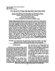
Segmenting this set of points into clusters of points which reside on the same algebraic surface is bene cial for the following reasons: 1. Removal of redundant information greatly simpli es the acquired data set and enables fast rendering and fast 3{D CAD modeling. 2. The points which lie on the intersection of the 3{ D surfaces are 3{D curves which can be utilized in registering the 3{D data set with 3{D or 2{D (images) data sets acquired from dierent locations in space. We are interested in estimating planar surface patches and 3{D lines at the locations where these patches intersect. This work can be extended towards the extraction of non-planar surface patches (polynomials of low degrees) and the localization of general 3{D curves instead of lines. We utilize the density of the range data and the organized way in which the data is measured by the range sensor. Our range measurements are very accurate and the segmentation can be very accurate as well. In gure 2 you can see the data ow of the planar segmentation and 3{D edge detection. We will describe each individual module in the following sections. We have built a mobile robot system which contains both range and image sensors which can be navigated to acquisition sites to create these site models (described in detail in [10]). The range data is registered wrt the image when a number of correspondences between the automatically extracted range and image edges is known. Thus we are calculating the relative position of the camera wrt the range sensor (translation and orientation). We believe that a hybrid approach which uses both range and image sensing can lead to very accurate results both photometrically and geometrically. Section 2 presents an overview of the related work. The extraction of planar surfaces and 3{D lines from range data and of 2{D lines from image data is the

FUSING GEOMETRIC WITH PHOTOMETRIC INFORMATION

Range Sensor

Organized set of Surface 3-D points fitting

Set of surfaces Intersection

PARTIAL 3D MODEL

2-D IMAGE

Real Curves 2-D Feature Extraction

Verification

Set of Curves

3-D Feature Extraction

2-D FEATURES (Lines)

3-D FEATURES (Planes and Lines)

MATCH

Figure 2: Flow for planar segmentation and 3{D edge detection.

REGISTRATION

Range Sensor

Cluster A

TEXTURE

MAPPING

Cluster B

P

A1

Rows

Cluster C

A3 FINAL PHOTOREALISTIC MODEL

A2

Cluster D

Columns

Figure 1: System for photorealistic 3{D modeling. topic of section 3. In section 4 we present the registration between range and image data. Section 5 presents the results of the algorithms on real data measured using the Cyra Scanner [6] in the Columbia University area (planar segmentation, 3{D edge detection, 2{D line detection, registration and texture mapping). Finally section 6 presents thoughts for future work.

2 Related work

In the area of range segmentation Besl and Jain in [4] describe an algorithm which ts bivariate{ polynomial surfaces of various degrees on the 3{D data. The algorithm is more general than our approach (we try to t planes only). However it is more computationally intensive and we believe that it is not suited for our large high{quality data. In [11] a comparison of many range segmentation algorithms is presented. Work in 3{D edge detection includes the algorithms presented in [13, 17]. In this case an edge{ following procedure is essential for the computation of 3{D lines. In our approach 3{D lines are produced directly at the intersection of the extracted planar surfaces. The extraction of photorealistic models of outdoor environments has received much attention recently. Including in this is the work of Shum [18], Becker

Figure 3: Sequential labeling. [1, 2], and Debevec [7]. Those methods use only 2{D images but the user guides the model creation phase. This leads to lack of scalability wrt the number of processed images of the scene and to the computation of simpli ed geometric descriptions of the scene. Teller [5, 16, 21] on the other hand acquires and processes a large amount of pose{annotated spherical imagery of the scene. However, this method suers from the large amount of information to be processed. Finally Zisserman's group in Oxford [9] works towards the fully automatic construction of graphical models of scenes when the input is a sequence of closely spaced 2{D images (video sequence). The problem in this case is the sparse depth estimates which depend on the texture and geometric structure of the scene. In our approach the use of range sensing provides dense geometric detail which lacks photometric information. We believe that we can create photorealistic models of high geometric and photometric detail by fusing 3{D range and 2{D image data. The VIT group [23, 3, 8] has built a mobile platform which carries a range and several camera sensors and acquire geometric and photometric information of indoor and outdoor scenes. This method is the closest to ours since it combines range with image sensing. The basic problem is the excessive use of sensors (nine cameras and a range sensor on the platform) in an ad{

hoc manner. The bundle adjustment procedure used for the registration between views is not guaranteed to work in all cases and the presented experimental results do not address this issue.

3 3{D & 2{D feature extraction 3.1

Planar surface extraction

We want to group the measured 3{D points into clusters of neighboring points which correspond to the same surface. Two points are considered neighbors if they are adjacent (8{connected) in the grid of measured 3{D points. The outline of our approach is the following: Point Classi cation A local plane is being t in the k  k neighborhood of every 3{D point. If the t is acceptable the point is classi ed as locally planar otherwise is classi ed as non{planar. Finally if the number of sensed points in the k  k neighborhood is not enough to produce a reliable t the point is classi ed as isolated. Cluster Initialization Create one cluster for every locally planar point. Cluster Merging Start with the upper left corner in the grid and sequentially visit all locally planar clusters (see gure 3). Final Planar Fit Perform a nal planar t on the points of each cluster. In the Point Classi cation phase a plane is t to the points vi which lie on the k  k neighborhood of every point P . The normal np of the computed plane corresponds to the smallest eigenvector of the 3 by 3 matrix A = Ni=1((vi m)T
(vi m)) where m is the centroid of the set of vertices vi. The smallest eigenvalue of the matrix A expresses the deviation of the points vi from the tted plane, that is it is a measure of the quality of the t. If the deviation is below a user speci ed threshold Pthresh the center of the neighborhood is classi ed as locally planar point. A list of clusters is initialized, one cluster per locally planar point. The next step is to merge the initial list of clusters and to create a minimumnumber of clusters of maximum size. Each cluster is de ned as a set of 3{D points which are connected and which lie on the same algebraic surface (plane in our case). We visit all the locally planar 3{D points sequentially (from left to right and from top to bottom ). We do not consider at all the non{locally planar and isolated points. For each point P we are visiting its three neighbors A1 ; A2 and A3 ( gure 3). We have to decide if the two points P and Aj could lie on the same planar

surface. If this is the case the clusters where those two points belong are merged into one new cluster. Two adjacent locally planar points are considered to lie on the same planar surface if their corresponding local planar patches have similar orientation and are close in 3D space.

n1 ,

P1

P1

n2 r12

P

,2

P2

Figure 4: Coplanarity measure. Two planar patches tted around points P1 and P2 at a distance jr12j. We introduce a metric of co{normality and co{ planarity of two planar patches. Figure 4 displays two local planar patches which have been t around the points P1 and P2 (Point Classi cation). The normal of the patches are n1 and n2 respectively. The points Pi0 are the projections of the points Pi on the patches. The two planar patches are considered to be part of the same planar surface if both conditions are met: 1. The patches have identical orientation (within a tolerance region), that is the angle  = cos 1 (n1
n2) is smaller than a threshold thresh [co{ normality measure]. 2. The patches lie on the same in nite plane [co{ planarity measure]. The distance between the two patches is de ned as d = max(jr12
n1j; jr12
n2j): This distance should be smaller than a threshold dthresh . Finally we t a plane on all points of the nal clusters. We also extract the outer boundary of this plane, the convex hull of this boundary and the axisaligned three-dimensional bounding box which encloses this boundary (used for fast distance computation between the extracted bounded planar regions; see next section). 3.2

3{D Line Detection

The intersection of the planar regions provides three dimensional lines. This is done in two stages: 1. We compute the in nite 3{D lines at the intersection of the extracted planar regions. We do not consider every possible pair of planar regions

but only those whose three-dimensional bounding boxes are close wrt each other (distance threshold dbound ). The computation of the distance between two bounding boxes is very fast. However this measure maybe inaccurate. Thus we may end up with lines which are the intersection of non-neighboring planes. 2. In order to lter out ctitious lines which are produced by the intersection of non-neighboring planes we disregard all lines whose distance from both producing polygons is larger than a threshold dpoly . The distance of the 3{D line from a convex polygon (both the line and the polygon lie on the same plane) is the minimum distance of this line from every edge of the polygon. In order to compute the distance between two line segments we use a fast algorithm described in [15]. We can verify the existence of the lines by checking if they pass through space which is occupied by measured 3{D points, but this test has not been implemented yet. 3.3

2{D line detection

The computation of 2{D linear image segments is done in the following manner: 1. Application of Canny edge detection with hysteresis thresholding. That provides chains of 2{D edges where each edge is one pixel in size (edge tracking). We used the program xcv of the TargetJr distribution [20] in order to compute the Canny edges. 2. Segmentation of each chain of 2{D edges into linear parts. Each linear part has a minimumlength of lmin edges and the maximum least square deviation from the underlying edges is nthresh . The tting is incremental, that is we try to t the maximum number of edges to a linear segment while we traverse the edge chain (orthogonal regression).

4 Registering range & image data

The problem we are attacking next is the fusion of the information provided by the range and image sensors. Those two sensors provide information of a qualitatively dierent nature and have distinct projection models. While the range sensor provides the distance between the sensed points and its center of projection, the image sensor captures the light emitted from scene points. The fusion of information between those two sensors requires the knowledge of the internal camera parameters (eective focal length, principal point

and distortion parameters) and the relative position and orientation between the centers of projection of the camera and the range sensor. The knowledge of those parameters allows us to invert the image formation process and to project back the color information captured by the camera on the 3{D points provided by the range sensor. Thus we can create a photorealistic representation of the environment. The estimation of the unknown position and orientation of an internally calibrated camera wrt the range sensor is possible if a corresponding set of 3{D and 2{D features is known. This corresponding set is provided by the user but the goal is its automatic computation (see section 6). Also the camera can self{calibrate (internal parameters) by utilizing the parallelism between straight lines in man{made scenes (see section 6). The types of features we are using for matching are 3{D range and 2{D image lines (sections 3.2 and 3.3). Corresponding lines are those which are produced by the same physical scene structure. The automated matching between 3{D and 2{D lines is complicated by the fact that 2{D edges are produced by depth, surface normal, lighting or re ectance discontinuities (geometric, material and lighting properties) whereas 3-D edges are the result of depth and surface discontinuities only (geometric properties). We adapted the algorithm proposed by Kumar & Hanson [14] for the registration between range and 2{ D images. The input is a set of corresponding 3{D and 2{D line pairs. The internal calibration parameters of the camera are assumed to be known. Let Ni be the normal of the plane formed by the ith image line and the center of projection of the camera ( gure 5). This vector is expressed in the coordinate system of the camera. The sum of the squared perpendicular distance of the endpoints e1i and e2i of the corresponding ith 3{D line from that plane is di = (Ni
(R(e1i ) + T))2 + (Ni
(R(e2i ) + T))2 ; (1) where the endpoints e1i and e2i are expressed in the coordinate system of the range sensor. The error function we wish to minimize is E1 (R; T) = Ni=1 di: (2) This function is minimized with respect to the rotation matrix R and the translation vector T. This error function expresses the perpendicular distance of the endpoints of a 3{D line from the plane formed by the perspective projection of the corresponding 2{D line into 3{D space ( gure 5). The exact location of the endpoints of the 2{D image segment do not contribute to the error metric and they can move freely along the

Ni

e1i

00 11 0 1 0 1 0 1

e2

11 00 00 11

Image Plane

i

3-D line

Distance of 3-D line’s endpoints from plane formed by corresponding 2-D line and camera’s center of projection.

Camera’s 1 0

2-D line

Coordinate System

Range Sensor’s Coordinate System

R, T

Figure 5: Error metric used for the registration of 3{D and 2{D line sets. image line without aecting the error metric. In this case we have a matching between in nite image lines and nite 3{D segments. The minimization of that metric is similar to the iterative technique proposed by Horn [12]. Let ei0 = Rei, where ei is a 3{D point expressed in the coordinate system of the range sensor. Then an incremental in nitesimal rotation d! will transform ei0 to ei00 = ei 0 + d!  ei0 :

(3)

Using this fact the application of an in nitesimal incremental rotation d! and an incremental translation dT would change the error metric to E1(R R(d!); T + dT):

(4)

By taking the derivatives of this error with respect to d! and dT and setting the results equal to 0 we reach a linear system of 6 equations with 6 unknowns (the elements of d! and dT). The solution of this system (d!, dT) provides updates for the rotation matrix R and the translation vector T. The rotation is represented as a unit quartenion in order to convert non-in nitesimal rotational estimates d! to valid rotational representations. That procedure is run iteratively until the error metric becomes smaller than a threshold or a maximum number of iterations is reached. The extraction of reliable and accurate 3{ D and 2{D features is very important for the accuracy of the nal registration.

5 Results

In this section results of the 3{D model acquisition, planar segmentation, 3{D line detection, 2{D line detection and registration between range and image data are presented.

The range data was captured by a CYRA range scanner [6]. The building shown in those results was captured at a resolution of 992 by 989 3D points. In gure 6a you can see the 2{D image of the acquired scene (building on Columbia University campus). The 992 x 998 3{D points are organized into a triangular mesh of points which is stored as an ACIS CAD model [19]. That 3{D model is shown in gure 6b. The planar segmentation of the 3{D data set follows. The result is displayed in gure 7a. The parameters used where Pthresh = 0:08, thresh = 0:04 degrees and dthresh = 0:01 meters (parameters de ned in section 3.1). The size of the neighborhood used to t the initial planes was 7 by 7. Dierent planes are displayed with dierent colors. The points which didn't pass the rst stage of the planar segmentation algorithm and have been classi ed as non{locally planar (section 3.1) are displayed as red. The automatically extracted 3{D lines shown in gure 7b lie on the intersection of the planes of gure 7a (thresholds used: dbound = 0:4 meters and dpoly = 0:2 meters, section 3.2). Figure 8a contains the extracted 2{D lines. The matching set of 2{D and 3{D lines, which is used for the registration between the 2{D and 3{D data sets, is shown in gures 8b and 8c . This set is selected by the user. The registration between the range and image data (estimation of translation and orientation between the range and image sensors) follows. We used Tsai's calibration algorithm[22] and computed the eective focal length (5.46mm) and principal point (196:8, 205:5) of the camera (image resolution was 400 by 400). Using the translation and orientation estimation of the camera we project the selected 3{D lines (shown in gure 8c) and all 3{D lines (shown in gure 7b) on the 2{D image ( gure 6a). The result is shown in gure 9. You can see that the 3{D lines are accurately projected on the 2{D image (note the windows and the back building that appears on the top of the scene). This result shows that the extracted 3{D and 2{D lines and the registration between the camera and range sensor are very accurate. Figure 6c shows the nal photorealistic model of the scene. This photorealistic model is provided by the mapping of the 2{D texture information 6a on the 3{D model 6b.

6 Discussion

We have implemented a system which combines dense depth measurements from a range sensor and image information from a camera in order to create a photorealistic model of the scene. We addressed the issues of 3{D and 2{D feature extraction and of the fusion of the gathered information. We would like to

Figure 6: a) Image of the scene, b) 3D model of the scene and c) Image texture-mapped on 3D model after the registration. sets of 3{D and 2{D features. Again the extraction of three directions of parallel 3{D lines (using the automated extracted 3{D line set) and the corresponding directions of 2{D lines (using the automated extracted 2{D line set) can be the rst step in that procedure. The knowledge of those directions can be directly used for the solution of the relative orientation between the two sensors. On the other hand extraction of pattern of lines that form windows (which are prominent in the 3{D line set) can lead to the computation of the translation between the two sensors.

References Figure 10: Extracted sets of 2{D lines which correspond to parallel 3{D lines. Each set of 2{D lines converges to a distinct vanishing point. The three large axes in the middle of the image point to the corresponding vanishing points.

[1] S. Becker and V. M. J. Bove. Semi{automatic 3{ D model extraction from uncalibrated 2{D camera views. In SPIE Visual Data Exploration and Analysis II, volume 2410, pages 447{461, Feb. 1995. [2] S. C. Becker. Vision{assisted modeling from model{ based video representations. PhD thesis, Massachusetts Institute of Technology, Feb. 1997. [3] J.-A. Beraldin, L. Cournoyer, et al. Object model creation from multiple range images: Acquisition, calibration, model building and veri cation. In Intern.

extend the system towards the direction of minimal human interaction. At this point the human is involved in two stages: a) the internal calibration of the camera sensor and b) the selection of the matching set of 3{D and 2{D features. We have implemented a camera self{calibration algorithm when three directions of parallel 3{D lines are detected on the 2{D image [2]. The automated extraction of lines of this kind is possible in environments of man{made objects (e.g. buildings) and a result can be seen in gure 10. More challenging is the automated matching between

[4] P. J. Besl and R. C. Jain. Segmentation through variable{order surface tting. IEEE Trans. on PAMI, 10(2):167{192, Mar. 1988. [5] S. R. Coorg. Pose Imagery and Automated Three{ Dimensional Modeling of Urban Environments. PhD thesis, MIT, Sept. 1998. [6] Cyra technologies. http://www.cyra.com. [7] P. E. Debevec, C. J. Taylor, and J. Malik. Modeling and rendering architecure from photographs: A hybrid geometry-based and image-based approach. In SIGGRAPH, 1996.

Conf. on Recent Advances in 3{D Dig. Imaging and Modeling, pages 326{333, Ottawa, Canada, May 1997.

Figure 7: a) Planar segmentation (dierent planes correspond to dierent colors), b) Extracted 3D lines: intersection of planar regions.

Figure 8: a) Extracted 2D lines (red), b)Selected 2D lines and c) Selected 3D lines (corresponding to the 2D lines).

Figure 9: a) Selected 3-D lines projected on the image after the registration, b) All 3-D lines projected on the image after the registration. [8] S. F. El-Hakim, P. Boulanger, F. Blais, and J.-A. Beraldin. A system for indoor 3{D mapping and virtual environments. In Videometrics V, July 1997. [9] A. W. Fitzgibbon and A. Zisserman. Automatic 3D model acquisition and generation of new images from video sequences. In Proc. of European Signal Processing Conf. (EUSIPCO '98), Rhodes, Greece, pages 1261{1269, 1998. [10] A. Gueorguiev, P. K. Allen, E. Gold, and P. Blair. Design, architecture and control of a mobile site modeling robot. In IEEE International Conference on Robotics & Automation, San Francisco, Apr. 2000. [11] A. Hoover, G. Jean-Baptise, X. Jiang, et al. An experimental comparison of range image segmentation algorithms. In IEEE Trans. on PAMI, pages 1{17, July 1996. [12] B. Horn. Relative orientation. International Journal of Computer Vision, 4:59{78, 1990. [13] X. Jiang and H. Bunke. Edge detection in range images based on scan line approximation. Computer Vision and Image Understanding, 73(2):183{199, Feb. 1999. [14] R. Kumar and A. R. Hanson. Robust methods for estimating pose and a sensitivity analysis. Computer Vision Graphics and Image Processing, 60(3):313{342, Nov. 1994.

[15] V. J. Lumelsky. On fast computation of distance between line segments. Information Processing Letters, 21:55{61, 1985. [16] MIT City Scanning Project. http://graphics.lcs.mit.edu/city/city.html. [17] O. Monga, R. Deriche, and J.-M. Rocchisani. 3D edge detection using recursive ltering: Application to scanner images. Computer Vision Graphics and Image Processing, 53(1):76{87, Jan. 1991. [18] H.-Y. Shum, M. Han, and R. Szeliski. Interactive construction of 3D models from panoramic mosaic. In CVPR, Santa Barbara, CA, June 1998. [19] Spatial Technology. http://www.spatial.com/. [20] TargetJr. http://www.esat.kuleuven.ac.be/~ targetjr/. [21] S. Teller, S. Coorg, and N. Master. Acquisition of a large pose-mosaic dataset. In CVPR, pages 872{878, Santa Barbara, CA, June 1998. [22] R. Y. Tsai. An eÆcient and accurate camera calibration technique for 3D machine vision. In IEEE Conference on Computer Vision and Pattern Recognition, pages 364{374, June 1986. [23] Visual Information Technology Group, Canada. http://www.vit.iit.nrc.ca/VIT.html.