Integration of shape constraints in data association filters Giambattista Gennari, Alessandro Chiuso, Fabio Cuzzolin, Ruggero Frezza Abstract— Many algorithms have been proposed in literature to deal with the tracking and data association problem. A common assumption made in the proposed algorithms is that the targets are independent. There are however many interesting applications in which targets exhibit some sort of coordination, they satisfy shape constraints. In the current work a general and well formalized method which allows to embed such constraints into data association filters is proposed. The resulting algorithm performs robustly in challenging scenarios.
I. I NTRODUCTION Tracking and data association are key problems in many interesting applications such as satellite surveillance systems, air defence, air traffic control, visual tracking and motion capture. All these applications deal with a set of points (or targets) moving in space and generating measurements of their positions. Tracking the points means estimating their state recursively over time starting from the observations. If all points are equal and they are not producing an identifying label when they generate the measurement of their position, the problem is associating measurements to trajectories. The data association problem is complicated further by false detections and missing data. There is an extensive literature on this problem and standard methods can be found for instance in [1]. These includes the popular JPDAF (joint probabilistic data association filter). In [7] the MHT (multi hypothesis trackers) have been introduced. In such techniques a target is described through a mixture of gaussian densities. Monte Carlo approaches have been recently adopted [13], [14] as well. Adaptive algorithms [12] have been proposed in order to cope with particular uncertainties such as the unknown inputs which typifies maneuvering targets. In multiple models based techniques [8] each target is described by a finite number of state space models. In the approaches proposed in literature targets are modelled independently. In some interesting applications there might be some sort of coordination between targets; for instance one might have a set of targets rigidly connected. Taking into account information about the coordinated motion would be of great help in solving data association. This work has been supported by ASI, EU and MIUR. Giambattista Gennari is with the Dipartimento di Ingegneria dell’Informazione, Universit`a di Padova, Via Gradenigo 6/A, 35131 Padova, Italy,
[email protected] Alessandro Chiuso is with the Dipartimento di Ingegneria dell’Informazione, Universit`a di Padova Via Gradenigo 6/A, 35131 Padova, Italy,
[email protected] Fabio Cuzzolin is with the Politecnico of Milano, Milano, Italy, cuz-
[email protected] Ruggero Frezza is with the Dipartimento di Ingegneria dell’Informazione, Universit`a di Padova Via Gradenigo 6/A, 35131 Padova, Italy,
[email protected]
Consider a group of coordinated points and assume that some of them are occluded or generate measurements which are similar to those generated by other points or to false detections. Their state can be better estimated exploiting the coordination and the measurements generated by the other points forming the given group. The motion of a rigid pattern is only one example of coordination. Think for instance to formations of robots or to points placed on articulated bodies or to a network of systems which operate to achieve a common task. Coordination is a natural concept for humans. Deriving a general model for arbitrary forms of coordination would allow to develop algorithms capable of recognizing and tracking reliably arbitrary coordinated groups. Unfortunately, obtaining such a model does not seem to be so simple. To simplify the problem we note that, in many cases, the measurements generated by points which would be intuitively classified as coordinated satisfy constraints which are invariant with respect to the motion. Start from a simple case of coordination, the rigid motion. Rigidly linked points exhibit constant distances and angles. These are a prior constraint on the positions of points which are characterized by such distances or angles in each instant of time. Similar considerations hold for non rigid sets of targets as well. Targets moving in formation are coordinated and group according to some strategy independently of motion. Each point could be represented by a node on a graph. An edge would be placed between two nodes if the corresponding points were close according to some norm in an appropriate function space. Such connectivity holds independently from the trajectories that such points follow in the space or equivalently it is a prior constraint on the points positions (from which the graph can be constructed at each instant of time). Finally, think to coordinated points forming a circle which spreads and contracts periodically. The law describing the distances between the points and the center of the configuration are prior constraints on the points positions. The prior constraints can be conveniently described by a probabilistic model. The latter allows for instance to describe non perfectly rigid configurations of points whose pairwise distances can be assumed to be distributed according to appropriate density functions. Motivated by all considerations above, we assume that a prior density function of the positions of points is given. The main result of the paper is a general method to embed such prior knowledge into standard tracking algorithms. An overall observation model which takes into account also
the past history of the measurements is obtained. Moreover a general procedure which allows to learn the prior density from appropriate data sequences is introduced. Such density embeds prior knowledge and hence its validity extends to arbitrary motions of the points which can be even quite different from those observed during the learning phase. In the sequel the motion invariant knowledge is called shape. The resulting algorithm copes robustly with quite unpredictable motions performed by points in presence of high numbers of false detections and of occlusions lasting several consecutive time steps. The current work is strictly related to [4], [2] where a constrained version of the JPDAF has been proposed for visual tasks. The main contribution of our approach is the general and well formalized way adopted to extend the standard tracking and data association techniques. Our approach differs substantially from [4], [2] for what concerns the occlusions as well. Moreover, a general learning methodology is introduced. The solution to the problem of missing data is also one of the main innovations brought to our previous work [3]. Some analogies with this work can be found in motion capture literature [9], [10]. The focus is, however, on specific and technical aspects of the human body tracking rather than on the development of a general and comprehensive methodology for tracking and data association problems capable to deal with general form of coordination. In [6] the coordination of point features placed on a human body is described by a a convenient probability density function of positions and velocities. The authors assume that the trajectories are provided by an appropriate tracking algorithm and such model is used for detection and labelling (recognition) of human parts. In [5] closely spaced targets are not considered independently in order to avoid track coalescence. However the problem solved and the proposed approach differ completely from those presented in this work. In [15] the coordination of a group of targets is described as a common bulk effect superposed on an independent motion for each individual target through an appropriate dynamical model. A particle filter is applied to such model in order to estimate the state over time. There are also applications in which the overall motion of the group is of interest rather than the trajectories of the single targets(see [16]). The paper is structured as follows: in section II a brief introduction to the tracking and data association problem and to the standard solutions is presented. An alternative expression for the likelihood of the observation is derived in order to deal with missing data. In section III the shape constraints are introduced. A particular expression for the prior density embedding the motion invariant knowledge well suited to deal with rigid and articulated bodies is presented. A general method which allows to learn such density from data is described. In section IV an overall observation model taking into account targets dynamics and shape constraints is introduced. In section
V such overall model is employed in the computation of the associations probabilities. The computation of such probabilities in presence of missing data is treated in some details. A Monte Carlo approach is adopted in order to estimate the positions of occluded points. In section VI the state estimation process is presented. A general method which allows to embed the Monte Carlo estimates into the Kalman filters in order to obtain the overall state estimates of occluded points is explained in some details. Finally, in section VII our methodology is tested on real data. The experiments performed demonstrate the validity of our approach. The developed algorithm performs robustly in presence of many false detections and occlusions lasting several time steps.
II. T RACKING AND DATA ASSOCIATION Let us consider the problem of tracking a set of points (or targets) moving in space generating unlabelled 1 measurements of their positions. We assume the i-th point can be described by a linear state space model of the form: ( xi (k + 1) = Fi · xi (k) + vi (k) (1) yi (k) = Hi · xi (k) + w(k) where xi and yi are respectively the state (for instance position and velocity) and measurable position of target i. The model and measurement noises vi and w are assumed to be white and zero mean gaussian distributed with covariances Q and R respectively. In order to estimate the state of the point i over time a Kalman filter is associated to the model (1). Assume a state estimate of each point is available at time k − 1. The state predictions for the next time step k can be computed using the standard Kalman formulas. At time k, a set of Mk unlabelled measurements z(k) = [z1 (k), ..., zMk (k)] is received. In what follows the time index k is dropped − whenever unnecessary and x ˆ− i and Pi denote the prediction of state xi (k) and its error covariance respectively given the measurements up to time k − 1. If the measurements were labelled, i.e. we knew which measurement is associated to which target, they could be used to update in the standard way the state predictions. To deal with unlabelled measurements it is customary [1] to introduce the association events (or hypothesis) θ ∈ Θ. Θ is the association space, i.e. the set of all possible ways to associate measurements to targets. According to an association θ, each measurement is either associated to a target or it is considered a false detection2 . The underlying assumption is that each target either generates one (and only one) measurement or it is occluded, i.e. it is not guaranteed that every target generates one measurement. 1 Unlabelled means that it is unknown from which point a given measurement has been generated. 2 In this case one usually says that it comes from clutter.
Given an association θ, j(i, θ) will denote the measurement associated to the point i or equivalently: yi = zj(i,θ)
p(y1 , ..., yN | Z − ) =
Conditionally on an association θ the estimate x ˆi,θ of the state xi and its error covariance Pi,θ are given by standard Kalman recursions associated to the model (1) driven by measurements zj(i,θ) . For convenience of notation, we shall denote with Kx (yi , R) and KP (R) respectively the state and covariance update3 given measurement yi (R is the covariance of the measurement noise w in (1)), i.e. x ˆi,θ = Kx (zj(i,θ) , R) will be the estimate of the state at time k given measurements up to time k and Pi,θ = KP (R) its error covariance for all hypothesis θ which associates a measurement to the point i. When the point i generates no measurement according to the hypothesis θ, its conditional state estimate will coincide with the prediction given by the Kalman filter, i.e. x ˆi,θ = − x ˆ− and P = P for all θ which assign no measurement i,θ i i to the point i. Finally, in order to iterate the procedure described above, one needs to compute an overall state estimate for each point. This can be done starting from the conditional state estimates in the following way. Each conditional state estimate is given a degree of reliability which is the posterior probability of the corresponding association event. Let us denote with Z k = {z(0), ..., z(k)}; in a Bayesian setting, i.e. when a prior p(θ) is given, each hypothesis θ has associated a posterior probability p(θ | Z k ) which can be computed according to [1]: k
p(θ | Z ) = =
the points are described independently by (1), the density p(y1 , ..., yN | Z − ) is given by:
k−1
c · p(z(k) | θ, Z ) · p(θ|Z c · p(z(k) | θ, Z k−1 ) · p(θ)
k−1
)
(2)
where c is a normalization constant. In what follows Z and Z − indicate Z k and Z k−1 respectively. An overall estimate x ˆi of the state xi and its error covariance Pi can be obtained as follows: X x ˆi = x ˆi,θ · p(θ | Z) θ X Pi = Pi,θ · p(θ | Z)+ (3) θ X + (ˆ xi,θ − x ˆi ) · (ˆ xi,θ − x ˆi )0 · p(θ | Z) θ
Expressions for the prior probability p(θ) and for the likelihood of the measurements p(z | θ, Z − ) are given in [1]. We introduce an alternative expression for p(z | θ, Z − ) which will be very useful do deal with missing data in section V. The output variables y1 , ..., yN are described by an appropriate density p(y1 , ..., yN | Z − ) which depends on the past history Z − of the observations. For instance, when filtering form.
p(yi | Zi− )
(4)
i=1
where p(· | Zi− ) is a Gaussian density of mean H · x ˆ− i , the predicted position of point i provided by the i-th Kalman filter, and covariance H · Pi− · H T + R. In the remaining part of this section a generic observation model p(y1 , ..., yN | Z − ) is considered and a general expression for the likelihood of measurements is derived. This will be adopted in section V whereby p(y1 , ..., yN | Z − ) has a more general form of (4) since relations among points will be taken into account. The likelihood p(z | θ, Z − ) can be factorized as follows: p(z | θ, Z − ) = p(zF | θ, Z − ) · p(zT | θ, Z − )
(5)
where zT and zF denote the true (generated by points) and false measurements according to the given association θ respectively which are assumed to be independent. p(zF | θ, Z − ) is usually taken uniform in the observed space. In order to compute p(zT | θ, Z − ) we proceed in the following manner. zT = {zj(i,θ) , i ∈ Dθ } where Dθ is the set of indices of all detected points (which have generated a measurement according to θ) and j(i, θ) is the measurement associated to point i in the current hypothesis θ, i.e. yi = zj(i,θ) . Denote with yDθ = zT the following set of equations: yDθ = zT : yi = zj(i,θ) i ∈ Dθ When all the N points are detected (i.e. Dθ = {1, ..., N }), p(zT | θ, Z − ) can be computed through p(y1 , ..., yN | Z − ) as follows: p(zT | θ, Z − ) = p(yDθ = zT | Z − )
(6)
Some complications arise when the generic point i is occluded and the corresponding output variable yi is unknown according to a given association θ. In order to deal with this problem the following solution is proposed. Denote with Mθ the set of occluded points according to a given θ and with yMθ their unknown positions: yMθ = {yi , i ∈ Mθ } The likelihood p(zT | θ, Z − ) can be computed as in (6) marginalizing over the positions yMθ of the missing points: Z − p(zT | θ, Z ) = p(yDθ = zT , yMθ | Z − )dyMθ (7) When the observation model is of the form (4) Y p(zj(i,θ) | Zi− ) p(yDθ = zT , yMθ | Z − ) = i∈Dθ
· 3 In
N Y
Y
i∈Mθ
p(yi | Zi− )
(8)
where c is a normalization constant and k · k denotes the L2 norm.
and the integration (7) yields: Y p(zT | θ, Z − ) = p(zj(i,θ) | Zi− ) i∈Dθ
which is the standard expression used in [1]. Equation (7) will be very useful in section V where a more complicated observation model is considered. In conclusion, from (7), (5) and (2), the posterior probability p(θ | Z) of a given association θ is given by: p(θ | Z) =c · p(θ) · p(zF | θ, Z − )· Z · p(yDθ = zT , yMθ | Z − )dyMθ
(9)
Standard expressions for p(θ) and p(zF | θ, Z − ) can be found in [1]. III. S HAPE CONSTRAINTS As anticipated in the introduction there might be some sort of coordination between targets; their spacial configuration may be conveniently described by an a priori probabilistic model of the form p¯(y1 (k), ..., yN (k))
(10)
which depends only on the relative positions and not on motion of the single targets. We say that (10) describes the shape constraints of the points. In the next sections a general methodology which allows to embed an arbitrary p¯(y1 , ..., yN ) into a tracking algorithm is proposed. In the remaining part of this section a particular expression for p¯(y1 , ..., yN ) which is useful to deal with rigid and articulated bodies is derived. Such expression will be used in the experiments presented in section VII. In order to construct the model p¯(y1 , ..., yN ) we start by choosing properties of the positions of points which can be reasonably described by prior constraints. If the points form rigid or articulated patterns pairwise distances between rigidly connected points are a reasonable choice. In real scenarios the configurations of points may not be perfectly rigid and therefore a probabilistic model is more suited. We assume the distance between point i and j can be modeled 2 by a gaussian density with mean µij and variance σij . It is convenient to introduce the set R of pairs of points whose distances are characterized by variances which are sufficiently small (the variances would be equal to zero if pairs were perfectly rigid). Let us define 2 1 (d−µ) 1 N (d | µ, σ 2 ) := √ e− 2 σ2 2πσ 2 The density p¯(y1 (k), ..., yN (k)) is chosen of the following form4 : Y 2 p¯(y1 (k), ..., yN (k)) = c· N (kyi (k)−yj (k)k | µij , σij ) (i,j)∈R
(11) 4 Even though ky (k) − y (k)k is always positive we still assume that i j it can be approximately described by a gaussian density.
2 The means µij and the variances σij can be learned from data in the following manner. A standard tracking algorithm (based on independent dynamics (1)) provides the trajectories of the points from which all the possible pairwise distances are computed. At a given instant of time, all past values of a given distance can be used to compute its mean and variance. Pairs of points whose distances exhibit a variance greater that a convenient threshold are no longer considered. At the end of the learning phase all pairs which have not been discarded form the set R and the corresponding means and variances are available. Meaningful results are obtained if the trajectories are sufficiently and persistently exciting [11].
IV. O BSERVATION MODEL In this section we introduce an overall observation model which combines (10) describing mutual configuration and (4) modeling separately target dynamics. We assume the overall observation model p(y1 (k), ..., yN (k) | Z − ) can be factored in two terms embedding (10) and (4) in the following form p(y1 (k), ..., yN (k) | Z − ) =c ·
N Y
p(yi (k) | Zi− )·
i=1
(12)
· p¯(y1 (k), ..., yN (k)) The observation model (12) takes into account all the available information and it is employed in the computation of the associations probabilities as explained in the next section. V. A SSOCIATIONS PROBABILITIES In order to compute the posterior probability (9) of a given association θ the likelihood (7) of the true measurements zT needs to be computed. Similarly to (8), the overall observation model (12) can be written as follows: Y p(yDθ = zT , yMθ | Z − ) = c · p(zj(i,θ) | Zi− )· ·
Y
i∈Dθ
p(yi |
Zi− )
· p¯(yDθ = zT , yMθ )
(13)
i∈Mθ
which substituted into (7) yields: Y p(zj(i,θ) | Zi− )· p(zT | θ, Z − ) = c · Z ·
Y
i∈Dθ
p(yi | Zi− ) · p¯(yDθ = zT , yMθ ) dyMθ
(14)
i∈Mθ
The integral in (14) is solved through a Monte Carlo approach. The reason is twofold. First, it is simple and consistent. Second, as a byproduct, it yields for free a set of fair samples from the posterior distribution of the occluded
points positions. This allows to compute mean and covariance and hence provides a natural gaussian approximation of the more complicated posterior as discussed in some details in the next section. Following Monte Carlo approach one draws an appropriate number Ns of independent and identically distributed samples: Y (n) (n) yMθ , {yi , i ∈ Mθ } ∼ p(· | Zi− ) n = 1, ..., Ns i∈Mθ
(15) and computes the n-th weight through the following expression: (n) π (n) = p¯(yDθ = zT , yMθ = yMθ ) (16) Finally, the integral is computed as follows: Z Y Ns X p(yi | Zi− ) · p¯(yDθ = zT , yMθ ) dyMθ ∝ π (n) n=1
i∈Mθ
(17)
and substituted in (14) yields p(zT | θ, Z − ). VI. S TATE ESTIMATION A Kalman estimator based on the model (1) is associated to each target. Consider a target i which is detected according to a given association θ. The corresponding measurement zj(i,θ) is used to update the i-th Kalman estimator as in standard methods (see section II). Nevertheless, the probability of the hypothesis θ is computed in a different way with respect to the standard approaches, i.e. taking into account the shape information encoded in p¯(y1 , ..., yN ) as explained in the previous section. The associations probabilities contribute to the computation of the overall state estimates (3) which hence depend on the shape information as well. Consider now a point i which generates no measurement according to the association θ. In the standard approaches the corresponding Kalman estimator cannot be updated and the conditional state estimates of point i coincide with its state predictions as explained in section II. When an appropriate prior density p¯(y1 , ..., yN ) is available, a better solution can be adopted. The conditional density p(yMθ | yDθ = zT , Z − ) of the occluded points positions yMθ given the detected ones yDθ and the past history Z − of the observations can be written as follows: p(yMθ | yDθ = zT , Z − ) =
p(yDθ = zT , yMθ | Z − ) p(yDθ = zT | Z − )
The probability p(yDθ = zT , yMθ | Z − ) is given by (13) and p(yDθ = zT | Z − ) does not depend on yMθ , hence the following expression holds: Y p(zj(i,θ) | Zi− )· p(yMθ | yDθ = zT , Z − ) ∝ ·
Y i∈Mθ
i∈Dθ
p(yi | Zi− ) · p¯(yDθ = zT , yMθ )
Q and noting that i∈Dθ p(zj(i,θ) | Zi− ) does not depend on yMθ , the following expression is finally derived: Y p(yMθ | yDθ = zT , Z − ) ∝ p(yi | Zi− )·¯ p(yDθ = zT , yMθ ) i∈Mθ
(18) The density p(yMθ | yDθ = zT , Z − ) is approximated (see (15) and (16) and recall factored sampling techniques) by the following set: (n)
{(yMθ , π (n) ), n = 1, ..., Ns }
(19)
Such set can be used to compute a gaussian approximation of the density p(yMθ | yDθ = zT , Z − ) which will be useful in order to compute the state estimates of occluded targets: Y ˆ y ,θ ) p(yMθ | yDθ = zT , Z − ) ' N (yi | yˆi,θ , Σ i i∈Mθ
ˆ y ,θ are the weighted sample means and coyˆi,θ and Σ i variances respectively computed starting from (19). The posterior density p(yMθ | yDθ = zT , Z − ) embeds all the available information: the predictions Zi− provided by the Kalman filters, the shape constraints p¯(·) and the measurements zT of the detected points (see equation (18)). ˆ y ,θ are the Hence, it is reasonable to say that yˆi,θ and Σ i estimates and the error covariances of the positions of occluded points according to a given hypothesis θ: ( yˆi,θ = E[H · xi | θ, zT , p¯, Zi− ] (20) ˆ y ,θ = V ar[H · xi | θ, zT , p¯, Z − ] Σ i
i
where xi is the state of point i and H is the output matrix in the state model (1). p¯ and Zi− indicate explicitly that the prior constraints and the predictions provided by the ˆ y ,θ . Kalman estimators are used to obtained yˆi,θ and Σ i ˆ y ,θ are the When H is the identity matrix yˆi,θ and Σ i conditional state estimate (according to θ) and the error covariance respectively. When H is not the identity matrix and it is not invertible (for instance in those cases in which both the position and velocity of a point are embedded in the state vector) the following solution can be adopted. Associate to the occluded point i an unknown fictitious measurement z = H · xi + w where w ∼ N (0, R) and R is unknown. Such measurement is supposed to be equivalent to the information given by p¯ and by the measurements zT of the detected points in the given association θ or more formally: ( E[H · xi |θ, zT , p¯, Zi− ] = E[H · xi |θ, z, Zi− ] (21) V ar[H · xi |θ, zT , p¯, Zi− ] = V ar[H · xi |θ, z, Zi− ] The conditional estimates of the state given the measurement z and the past history Zi− are given by the Kalman estimator: ( E[H · xi |θ, z, Zi− ] = H · Kx (z, R) (22) V ar[H · xi |θ, z, Zi− ] = H · KP (R) · H T
where Kx (z, R) and KP (R) indicate the state estimate and the relative error covariance provided by the estimator (see section II) whose explicit expressions are the following: ( Kx (z, R) = x ˆ− + P − H T Λ−1 · e (23) KP (R) = P − − P − H T Λ−1 HP − x ˆ− and P − are the state prediction and the corresponding error covariance, e = z − Hx− is the innovation and Λ is the innovation covariance which is given by the following expression: Λ = HP − H T + R
Fig. 1. On the left hand side a picture of the scene is reported. Five points are placed on the cover of a book. Many points are located on other objects. On the right hand side the overall set of observations at a given instant of time is depicted (the measurements of the five points on the book are highlighted). Tracking with no shape information (target 5)
where the subscripts i and θ are dropped for convenience of notation. Using (23) in (24) yields ( yˆ = H x ˆ− + SΛ−1 e (25) ˆ y = S − SΛ−1 S Σ where S = HP − H T . From the second equation of (25) follows that ˆ ξ S −1 ) Λ−1 = S −1 (I − Σ (26) (I is the identity matrix) which is meaningful under the following condition:
Tracking with shape information (target 5)
1.1
1.1
1.05
1.05
1
1
0.95
0.95
0.9 y [m]
0.9 y [m]
In order to obtain the state estimate Kx (z, R) and the corresponding error covariance KP (R) the unknowns quantities Λ−1 and e need to be computed. From equations (20), (21) and (22) follows that ( yˆ = H · Kx (z, R) (24) ˆ y = H · KP (R) · H T Σ
0.85
0.85
0.8
0.8
0.75
0.75
0.7
0.7
0.65
0.65
0.6
0
100
200
300
400
500 frame
600
700
800
900
1000
0.6
0
100
200
300
400
500 frame
600
700
800
900
1000
Fig. 2. The trajectory of the y-coordinate of a point of interest. At first, shape is not embedded into the tracker. The point is given many labels because the tracker is distracted by the measurements generated by other points. Moreover, an occluded point cannot be tracked reliably for many frames and it is given a new label when it is detected again. The segments of the point trajectory identified by many different labels are manually merged together and reported on the left hand side. Vertical lines indicate the time instants in which the point is given a new label. Note that in certain intervals of time the trajectory is not available since the point is occluded. When shape information is considered the tracker reconstructs reliably the trajectory of the point which is reported on the right hand side.
VII. E XPERIMENTS
The algorithm is tested on real data obtained through a motion capture system. Points on a rigid body are moving Substituting (26) in the first equation of (25) yields the in space and generating measurements of their positions. Many other observations are generated by other points (see expression for the innovation: figure (1)). Moreover some of the points of interest can be ˆ y S −1 )−1 (ˆ e = (I − Σ y − Hx ˆ− ) (27) occluded for several frames. The dynamics of targets are described by (1) where the state Using (26) and (27) in (23) yields the expression of the of each point is formed by its position and velocity. The state estimate shape model is of the form (11) and it is learned from data − − T −1 −1 −1 −1 ˆ y S )(I − Σ ˆ y S ) · as explained in section III. The algorithm performs robustly. Kx (z, R) = x ˆ + P H S (I − Σ The state estimates are not affected by the many observa· (ˆ y − Hx ˆ− ) tions close to those generated by the points of interest. The =x ˆ− + P − H T (HP − H T )−1 (ˆ y − Hx ˆ− ) trajectories of occluded points are reconstructed reliably. The tracking algorithm does not exhibit such robustness = Kx (ˆ y , R = 0) when shape knowledge is not considered (see figure (2)). In and of the estimate error covariance: absence of shape one could improve performances adopting − − T − T −1 − T −1 ˆ y (HP H ) ]· for instance multi hypothesis techniques. However, many KP (R) = P − P H (HP H ) [I − Σ measurements which are not generated by targets of interest · HP − are persistently present in the observed space. This implies = P − − P − H T (HP − H T )−1 HP − + P − H T S −1 · in general many and persistent hypothesis (i.e. high ambiguity) on the state of a given point of interest. Moreover, ˆ y S −1 HP − ·Σ when shape is not available, it is not possible to reconstruct ˆ y S −1 HP − = KP (R = 0) + P − H T S −1 Σ the trajectories of occluded targets even using sophisticated ˆ y < HP − H T Σ
tracking algorithms. Also computational aspects have been examined. The bottleneck of the algorithm could be considered the Monte Carlo computations performed to deal with missing points. In order to reduce the number of times numerical integration has to be solved hypothesis that a certain target is occluded are considered only if there are no other associations where it is matched to some measurement which have a reasonably high likelihood. VIII. C ONCLUSIONS AND FUTURE WORK A general and well formalized methodology which allows the integration of prior probabilistic shape constraints into data association filters has been presented. Such methodology is flexible since the shape prior can be of arbitrary form. Moreover, shape constraints can be learned from data and their validity extends to arbitrary motions. A general and comprehensive solution to the problem of missing data is given. The resulting algorithm performs robustly in presence of many false detections and occlusions lasting several consecutive time steps. Short term future work concerns the on line learning of shape constraints which is done embedding the learning phase into the tracking process. This would eliminate the off line learning which requires sufficiently and persistently exciting data sequences without heavy clutter and long occlusions. Clearly, prior information implies great robustness and hence it should be used whenever possible. A long term goal is the derivation of a general description of coordination which would lead to the development of powerful tracking algorithms capable of recognizing and tracking groups of targets exhibiting arbitrary forms of coordination. R EFERENCES [1] Y. Bar-Shalom and T.E. Fortmann “Tracking and data association”, New York, Academic Press, 1988. [2] C. Rasmussen, G.D. Hager, Probabilistic Data Association Methods for Tracking Complex Visual Objects, IEEE Trans. on Pattern Analysis and Machine Intelligence, Vol. 23, No.6, June 2001, pp. 560-576. [3] G. Gennari, A. Chiuso, F. Cuzzolin, R. Frezza, ”Integrating probabilistic shape and dynamic models in data association and tracking”, Proc. IEEE Int. Conf. on Decision and Control, Las Vegas, 2002. [4] C. Rasmussen G. D. Hager, ”Joint Probabilistic Techniques for tracking multi-part objects”, Proc. Computer Vision and Pattern Recognition, 1998, pp. 16-21. [5] Henk A. P. Blom and Edwin A. Bloem, Probabilistic Data Association Avoiding Track Coalescence, IEEE Trans. on Automatic Control, Vol. 45, No. 2, Febraury 2000, pp. 247-259. [6] Yang Song, Luis Goncalves and Pietro Perona, ”Monocular perception of biological motion-clutter and partial occlusion”, Proc. of European Conference of Computer Vision, June 2000. [7] Donald B. Reid, An algorithm for tracking multiple targets, IEEE Trans. on Automatic Control, Vol. 24, No. 6, pp. 843-854, 1979. [8] E. Mazor, A. Averbuch, Y. Bar Shalom, J. Dayan, Interacting Multiple Model Methods in Target Tracking: A survey, IEEE Trans. on Aerospace and Electronic systems, Vol. 34, No. 1, January 1998, pp. 103-123.
[9] M. Ringer and J. Lasenby, ”Multiple Hypothesis Tracking for Automatic Optical Motion Capture”, European Conf. on Computer Vision, 2002, pp. 524-536. [10] L. Herda, P. Fua, R. Plankers, R. Boulic and D. Thalmann, SkeletonBased Motion Capture for Robust Reconstruction of Human Motion, Computer Animation, IEEE press, May 2000. [11] L.Ljung, System identification : theory for the user, Prentice Hall, 1997. [12] Y. Bar-Shalom and X.R. Li “Multitarget-Multisensor Tracking: Principles and techniques”. YBS Publishing, 1995. [13] Carine Hue, Jean-Pierre Le Cadre, Patrick Perez, Sequential Monte Carlo Methods for Multiple Target Tracking and Data Fusion, IEEE Trans. on Signal Processing, Vol. 50, No.2, February 2002, pp. 309325. [14] A. Doucet, B-N. Vo, C. Andrieu, and M. Davy, ”Particle filtering for multi-target tracking and sensor management”, International Conference on Information Fusion, Vol. 1, pp. 474–481, 2002. [15] D.J. Salmond, N.J. Gordon, ”Group Tracking with limited sensor resolution and finite field of view”, SPIE Proc. of Signal and Data Processing of Small Targets, Vol. 4048, pp. 532-540, 2000. [16] Ron Mahler, Tim Zajic, ”Bulk Multitarget Tracking Using a FirstOrder Multitarget Moment Filter”, SPIE Proc. of Signal Processing, Sensor Fusion and Target Recognition, Vol. 4729, pp. 175-186, 2002