Integration Testing of Software Product Lines Using ... - UNL CSE

Integration Testing of Software Product Lines Using Compositional Symbolic Execution Jiangfan Shi, Myra B. Cohen and Matthew B. Dwyer Dept. of Computer Science & Engineering University of Nebraska-Lincoln Lincoln, NE 68588-0115

Abstract. Software product lines are families of products defined by feature commonality and variability, with a well-managed asset base. Recent work in testing of software product lines has exploited similarities in different development phases to reuse shared assets and reduce test effort. The use of feature dependence graphs has also been employed, and there has been some work that aims to reduce duplication of partial products during integration testing, but less that focuses on code level analysis of dataflow between features. In this paper we present a compositional symbolic execution technique that works in concert with a feature dependence graph to extract the set of possible interaction trees in a product family. It then composes these to incrementally and symbolically analyze feature interactions. We experiment with two product lines and determine that our technique can reduce the overall number of interactions that must be considered during testing, and requires less time to run than a traditional directed symbolic execution technique.

1

Introduction

Software product line (SPL) engineering is a methodology for developing families of software programs through the managed reuse of a common and variable set of assets [19]. Variability at the application level is expressed in terms of features (functional units) that are included or excluded from the individual programs. The result is a set of similar, but unique program instantiations. While uniqueness arises from the different combination of variable features in each program, similarity comes from both the commonality found in all instantiations, as well as from matching subsets of features (i.e. partial products) between programs. Variability, and the ability to generate many products from a core set of features, provides flexibility and leverages reuse during development, but causes problems for validation. Although individual features may be validated and tested in multiple programs within the product line, this does not guarantee that specific combinations of features will work properly when composed. Research has shown that some faults – termed interaction faults – only occur under specific combinations of features [3, 14] and several SPL testing techniques have attempted to account for this. For instance, Bertolino et al. [1] and Geppert et al. [2] propose a specification based technique to concretize a parameterized use

2

Jiangfan Shi, Myra B. Cohen and Matthew B. Dwyer

case (based on variability), but this is an exhaustive approach that tests each product individually. This is a limitation, since the variability space grows exponentially with the number of features. Suppose we have 4 choices for each of 10 features. To test all possible combinations of features, we need to test 410 or 1, 048, 576 instantiation which may be infeasible. Kim et al. [12] use a dependency analysis to determine which features are relevant for each test within a test suite, reducing the number of products tested per test case. This technique does not consider coverage of the entire feature model, nor does it target the specific interactions; it only reduces the per-test number products. A study by Reisner et al. [21] shows that in some configurable systems – SPLs can be viewed as a type of configurable software system – analysis of control flow can reduce the possible set of configuration options that should be tested together. They do not consider other types of dependencies such as data flow, nor do they apply their approach to product lines. And neither of these studies targets specific interactions for test generation; they only reduce the number of feature combinations that should not be tested together. In our earlier research [4], we proposed a mapping between the variability space of an SPL and a relational model in order to leverage ideas from combinatorial interaction testing (CIT), a model-based sampling technique that guarantees to test all pairs or t-way combinations of features within the product line. Instead of testing all program instantiations in the example above, we can test all pairs of features with approximately 24 SPL instances, or all triples of features with around 130, using a common CIT generation tool [3]. Since empirical evidence suggests that lower order interactions are responsible for most interaction faults this provides some justification for CIT sampling [14]. While CIT provides a notion of coverage of the variability space, it also suffers from limitations. First, there is an expectation that all possible programs in the product line can be composed. But there may be features or groups of features that are not developed until later phases of the SPL lifetime. Second, since CIT operates at the feature combination level there is no guarantee that testing of an instance will execute the interacting code; this will depend on the quality of the test. Finally, CIT does not consider the direction of the interactions in its model, yet at the code level, interactions may happen between features in different directions. For instance if we have three features (f1 , f2 , f3 ), there are six directed 2-way interactions possible between these features. When testing a software product line to uncover interactions, we should test from a perspective that avoids these limitations. Uncovering interactions during integration testing – where features are composed as partial products – appears to make sense from a combinatorial sense. We can test only the interactions themselves and combine products in a way that avoids redundancy. Uzuncaova et al. [25] use this idea by reusing a partial product’s integration test results to generate a smaller test suite for a larger partial product. And Reis et al. [20] apply integration testing over an SPL at the specification level to avoid redundantly testing common partial products. Finally, Stricker et al. [24] present

Integration Testing of SPLs

3

the ScenTED-DF methodology which uses dataflow between products to drive integration testing at the model level. In this paper we present a new method of integration testing for software product lines aimed at identifying at the dataflow level of abstraction, interactions between features. We use ideas from CIT to drive coverage of feature interaction tuples. We reduce the variability space through the use of a codebased dependency analysis resulting in a set of directed interaction trees that define the patterns of interactions possible between features for each interaction level (i.e. pairs, triples, . . ., k-tuples). We then use symbolic execution to evaluate each tree compositionally. The result is a method that generates constraints for all partial products at a lower cost than a full symbolic execution of an SPL code base. We also find, that by counting directed interactions, we have a more precise model of what should be tested. Finally, if we consider the constraints arising from symbolic execution, these can be used to inform a test generation technique to focus on the parts of the system that may have faults. The contributions of this work are: (1) a dataflow informed compositional symbolic integration testing method for SPLs; (2) the first discussion of interaction testing that incorporates directions; and (3) a feasibility study that shows we can reduce the number of interactions to test, and that the compositional technique uses less time than traditional symbolic execution.

2 2.1

Background Feature Models

Software product lines are families of software systems designed for a specific domain, with a managed set of assets and well defined variability model [19]. The products all share some commonality, but are customized by variable elements of the system. Product lines vary in when they are configured. Some may be configured by the developer at build time, others allow changes through recompilation, while some use run-time constructs to change during execution. A key artifact of a software product line is the feature (or variability) model. This is one differentiator from a general configurable system. There are many formalisms that have been developed to represent these. In this paper we use the Orthogonal Variability Model (OVM) developed by Pohl et al. [19]. In OVM Variation points (VP) are shown as triangles and variants (v) are shown as rectangles. Variants will map directly to features in this paper. Dependencies are shown as solid lines (mandatory) or dashed (optional). Alternative choices are shown with arcs which are annotated with the the minimum and maximum cardinality of that VP. When there is no annotation, exactly one variant can be selected for the variation point. Additional constraints are allowed between parts of the model in the form of excludes or requires.

4

2.2


Symbolic Execution

Symbolic execution [13] is a path-sensitive program analysis technique that computes program output values as expressions over symbolic input values and constants. Symbolic execution of the code fragment: y = x; if (y > 0) then y++; return y; would use a symbolic value X to denote the value of variable x on entry to the fragment. Symbolic execution determines that there are two possible paths (1) when X > 0 the value X + 1 is returned and (2) when !(X > 0) the value X is returned. The analysis represents the behavior of the fragment as the pairs (X > 0, RETURN == X + 1) and (!(X > 0), RETURN == X). The first element of a pair encodes the conjunction of constraints along an execution path – the path condition. The second element defines the values of the locations that are written along the path in terms of the symbolic input variables, e.g. RETURN == X means that the original value for x is returned. The state of a symbolic execution is a triple (l, pc, s) where l, the current location, records the next statement to be executed, pc, the path condition, is the conjunction of branch conditions encoded as constraints along the current execution path, and s : M × expr is a map that records a symbolic expression for each memory location, M , accessed along the path. Computation statements, m1 = m2 m3 , where the mi ∈ M and is some operator, when executed symbolically in state (l, pc, s) produce a new state (l + 1, pc, s0 ) where ∀m ∈ M − {m1 } : s0 (m) = s(m) and s(m1 ) = s(m2 ) s(m3 ). Branching statements, if m1 m2 goto d, when executed symbolically in state (l, pc, s) branch the symbolic execution to two new states (d, pc∧s(m1 ) s(m2 ), s) and (l + 1, pc ∧ ¬(s(m1 ) s(m2 )), s) corresponding to the “true” and “false” evaluation of the branch condition, respectively. An automated decision procedure is used to check the satisfiability of the updated path conditions and, when a path condition is found to be unsatisfiable, symbolic execution along that path halts. Decision procedures for a range of theories used to express path conditions, such as, linear arithmetic, arrays, and bit-vectors are available, e.g., Z3 [6]. 2.3

Symbolic Method Summary

Several researchers [9, 18] have explored the use of method summarization in symbolic execution. In [9] summarization is used as a mechanism for optimizing the performance of symbolic execution whereas [18] explores the use of summarization as a means of abstracting program behavior to avoid symbolic execution. We adopt the definition of method summary in [18], but we forgo their use of over-approximation. The building block for a method summary is the representation of a single execution path through method, m, encoded as the pair (pc, w). This pair provides


$#

12# "*"#

!"#

&

% !'#

!(#

345# !"# !(# "*'#

!'#

!)#

s() {! f1(){! …! …! }! v();! if (c) {! f (){! 2 …! …! }! }! w();! f3() ! …! }! f4() !

78/9-+#680+#

• K+L89 1, we can define a pair of interaction trees ti = (Fi , Ei ) and tj = (Fj , Ej ), such that Fi ∩ Fj = ∅, |Fi | + |Fj | = k, and ∃(fi , fj ) ∈ E. We say that tk is the parent of ti and tj and, conversely, that ti and tj are the children of tk . The base case of the hierarchy, where k = 1, is simply each feature in isolation. There are many ways to construct such an interaction hierarchy, since for any given k-way interaction tree cutting a single edge partitions the tree into two children. As discussed below, the hierarchy resulting from Algorithm 1 enjoys

8


Algorithm 1 Computing k-way Interaction Trees interactionTrees(k, (F, E)) T := ∅ for (fi , fj ) ∈ E T ∪ = tree(fi , fj ) for i = 3 to k + 1 for ti−1 ∈ T ∧ |ti−1 | = i − 1 for v ∈ F − v(ti−1 ) if (root(ti−1 ), v) ∈ E ∧ consistent(v(ti−1 ∪ v) then T ∪ = tree(ti−1 , (root(ti−1 ), v)) else for (v, v 0 ) ∈ E ∧ v 0 ∈ v(ti−1 ) if consistent(v(ti−1 ∪ v) then T ∪ = tree(ti−1 , (v, v 0 )) endif return T end interactionTrees()

a structure that can be exploited in generating summaries of interaction pattern behavior. The parent (child) relationships among interaction trees can be recorded at the point where the tree() constructor calls are made in Algorithm 1. 3.3

Composing Feature Summaries

Our goal is to analyze program paths that span sets of features in an SPL to support fault detection and test generation. Our approach to feature summarization involves two distinct phases: (1) the application of bounded symbolic execution to feature implementations in isolation to produce feature summaries, and (2) the matching and combination of feature summaries to produce summaries of the behavior of interaction patterns. Phase (1) is performed by applying traditional symbolic execution where the length of the longest branch sequence is bounded to d – the depth. For each feature, f , this results in a summary, fsum , as defined in Section 2. When performing symbolic execution of f there are three possible outcomes: (a) a complete execution of f which returns normally as analyzed within d branches, (b) an exception, including assertion violations, is detected before d branches are explored, and (c) the depth bound is reached. In our work, we only accumulate the outcomes falling into (a) into fsum . Case (b) is interesting, because it may indicate a fault in feature f . The isolated symbolic execution of f allows for any possible state on entry to the feature, however, it is possible that a detected exception is infeasible in the context of a system execution. In future work, we will preserving results from case (b) and attempt to determine their feasibility when composed in interaction patterns with other features – this would reduce and, when interaction patterns are sufficiently large, eliminate false reports of exceptions. For phase (2) we exploit the structure of the interaction hierarchy resulting from the application of Algorithm 1 to generate a summary for a k-way interaction. As discussed above, such an interaction has (potentially several) pairs of children. It suffices to select any of those pairs.


9

Within each pair there is a k − 1-way interaction, i, which we assume has a summary isum = (pci , wi ), and single feature, f , summarized as fsum = (pcf , wf ), which is connected by a single edge connected to either root(i) or one of i’s leaves, l. To compose isum and fsum we must characterize the behavior of the FDG edge. The existence of an edge (f, f 0 ) means that there is a common region beginning at the return from f and ending at the call to f . Calculating the chop that circumscribes the CFG for this region allows us to label branch outcomes that lie within the chop and to direct the symbolic execution along paths from f that reach f 0 . Algorithm 2(left) defines this approach to calculating edge summaries. It consists of a customized depth-bounded symbolic execution that only explores a branch if that branch lies within the chop for the common region. The algorithm makes use of several helper functions. Functions determine whether an instruction is a branch, branch(), the target of a branch, target(), and the symbolic expression for a branch given a symbolic state, cond(). Functions to calculate the successor of an instruction, succ(), the set of locations written by an instruction, write(), and updating the symbolic state based on an instruction, update(), are also used. The SAT () predicate determines whether a logical formula is satisfiable. Finally, the π() function projects a symbolic state onto a set of locations. eSum(Echop , succ(f ), f 0 , true, ∅, ∅, d) returns the symbolic summary for edge (f, f 0 ) where the parameters are as follows. Echop is the set of edges in the CFG chop bounded by the return of f and the call to f 0 , succ(f ) is the location at which initiate symbolic execution and f 0 is the call that terminates symbolic execution. true is the initial path condition. The next two parameters are the initial symbolic state and the set of locations written on the path – both are initially empty. d is the bound on the length of the path condition that will be explored in producing the summary. To produce a symbolic summary for the k-way interaction, we now compose isum , fsum , and the edge summary computed by eSum(). There are two cases to consider. If the feature, f 0 , is connected to root(i) with an edge, (root(i), f 0 ) 0 . If the we compose summaries in the following order: isum , (root(i), f 0 )sum , fsum 0 0 feature, f , is connected to a leaf of i, li , with an edge, (f , li ) we compose 0 summaries in the following order: fsum , (f 0 , li )sum , isum . Order matters in composing summaries because the set of written locations of two summaries may overlap and simply conjoining the equality constraints on the values at such locations will likely result in constraints that are unsatisfiable. In our composition approach, we honor the sequencing of writes and reads of locations that arise due to the order of composition. Consider the composition of summary s with summary s0 , in that order. Let (pc, w) ∈ s and (pc0 , w0 ) ∈ s0 be two elements of those summaries. The concern is that dom(w) ∩ dom(w0 ) 6= ∅, where dom() extracts the set of locations used to index into a map. Our goal is to eliminate the constraints in w on locations in dom(w) ∩ dom(w0 ). In general, pc0 will read the value of at least one location, l, and that location may have been written by the preceding summary.

10


Algorithm 2 Edge Summary (left) and Composing Summaries (right) eSum(E, l, e, pc, s, w, d) if |pc| > 0 cSum(s, s0 ) if branch(l) sc := ∅ lt := target(l, true) for (pc, w) ∈ s if SAT (cond(l, s)) ∧ (l, lt ) ∈ E for (pc0 , w0 ) ∈ s0 eSum(E, lt , e, pc ∧ cond(l, s), s, w, d − 1) eq := true lf := target(l, f alse) for l ∈ read(pc0 ) if SAT (¬cond(l, s)) ∧ (l, lf ) ∈ E if ∃l ∈ dom(w) eSum(E, lf , e, pc ∧ ¬cond(l, s), s, w, d − 1) eq := eq ∧ input(s0 , l) = w(l) else if SAT (pc ∧ eq ∧ pc0 ) if l = e for l ∈ dom(w0 ) sum ∪ = (pc, π(s, w)) if ∃l ∈ dom(w) else w := w − (l, ) s := update(s, l) endfor w ∪ = write(l) sc ∪ = (pc ∧ eq ∧ pc0 , w ∧ w0 ) eSum(E, succ(l), e, pc, s, w, d) endif endif endfor endif end cSum() if pc = true return sum end eSum()

In such a case, the input value referenced in pc0 should be equated to w(l). Algorithm 2(right) composes two summaries taking care of these two issues. In our approach, the generation of a symbolic summary produces “fresh” symbolic variables to name the values of inputs. A map, input(), records the relationship between input locations and those variables. We write input(s, l) to denote a summary s and a location l to access the symbolic variable. For a given path condition, pc, a call to read(pc) returns the set of locations referenced in the constraint – it does this by mapping back from symbolic variables to the associated input locations. We rely on these utility functions in Algorithm 2(right). The algorithm considers all pairs of summary elements and generates, through the analysis of the locations that are written by the first summary and read by the second summary, a set of equality constraints that encode the path condition of the second summary element in terms of the inputs of the first. The pair of path conditions along with these equality constraints are checked for satisfiability. If they are satisfiable, then the cumulative write effects of the summary composition are constructed. All of the writes of the later summary are enforced and the writes in the first that are shadowed by the second are eliminated – which eliminates the possibility of false inconsistency.

3.4

Complexity and Optimizion of Summary Composition

From studying the Algorithm 2 it is apparent that the worst-case cost of constructing all summaries up to k-way summaries is exponential in k. This is due to the quadratic nature of the composition algorithm.


11

In practice we see quite a different story, in large part because we have optimized summary composition significantly. First, when we can determine that a pair of elements from a summary that might potentially match we ensure that for any shared features the summaries agree on the values for the elements of those summaries; this can be achieved through a string comparison of the summary constraints which is much less expensive than calling the SAT solver. Second, we can efficiently scan for constraints in one summary that are not involved in another summary and those can be eliminated since they were already found to be satisfiable in previous summary analyses.

4

Case Study

We have designed a case study for evaluating the feasibility of our approach that ask the following two research questions. (RQ1): What is the reduction from our dependency analysis on the number of interactions that should be tested in an SPL? (RQ2): What is the difference in time between using our compositional symbolic technique versus a traditional directed technique? 4.1

Objects of Analysis

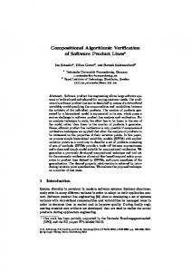
We selected two software product lines. The first SPL is based on the implementation of the Software Communication Architecture-Reference Implementation (SCARI-Open v2.2) [5] and the second is a graph product line, GPL [12,15] used in several other papers on SPL testing. The first product line, SCARI, was constructed by us as follows. First we began with the Java implementation of the framework. We removed the nonessential part of the product line (e.g. logging, product installation and launching) and features that required CORBA Libraries to execute. We kept the core mandatory feature, Audio Device, and transformed four features that were written in C (ModFM, DemodFM, Chorus and Echo), into Java. We then added 9 other features which we translated from C to Java from the GNU Open Source Radio [8] and the Sound Exchange (SoX), site [23]. Table 1 shows the origin of each feature and the number of summaries for each. We used the example function for assembling features, to write a configuration program that composes the features together into products. The feature model is shown in Figure 2(a).

!"#$%&'()$$

!*#$+,-$

Fig. 2. Feature Models for (a) SCARI and (b) GPL

12


Features Chorus Contrast Volume Repeat Trim Echo Reverse Fade Swap AudioDevice ModFM ModDBPSK DemodFM DemodDBPSK

Origin LOC No. Summaries [5] 30 6 [23] 14 5 [23] 47 5 [23] 12 3 [23] 11 6 [5] 31 5 [23] 14 4 [23] 9 4 [23] 27 4 [5] 13 3 [5] 19 4 [8] 6 2 [5] 18 4 [8] 6 3

Total

257

58

Table 1. SCARI Size by Feature

Features LOC No. Summaries Base 85 56 Weighted 32 148 Search 35 19 DFS 23 41 BFS 23 6 Connected 4 8 Transpose 27 3 StronglyConnected 19 9 Number 2 2 Cycle 40 19 MSTPrim 92 4 MSTKruskal 106 3 Shortest 102 3 Total

590

321

Table 2. GPL Size by Feature

The graph product line (GPL) [15] has been used for various studies on SPLs. We start with the version found in the implementation site for [12]. To fit our prototype tool, we re-factored some code so that every feature is contained in a method. We removed several features because either we could not find a method in the source code or because JPF would not run. We made the method Prog our main entry point for the program. We did not include any constraints for simplicity. Figure 2 shows the resulting feature model and Table 2 shows the number of lines of code and the number of summaries by feature. 4.2

Method and Metrics

Experiments are run on an AMD Linux computing cluster running CentOS 5.3 with 128GB memory per node. We use Java Pathfinder (JPF) [16] to perform SE with the Choco solver for SCARI and CVC3BitVector for GPL. We adapt the information flow analysis (IFA) package [10] in Soot [26] for our FDG. In SCARI we use the configuration program for a starting point of analysis. In GPL we use the Prog program, which is an under-approximation of the FDG. For RQ1 we compute the number of possible interactions (directed and undirected) at increasing values for k, obtained directly from the feature model. We compare this with the number that we get from the interaction trees. For RQ2, we compare the time that is required to execute the two symbolic techniques on all of the trees for increasing values of k. We compare incremental SE (IncComp) and a full direct SE (DirectSE). We set the depth for SE at 20 for IncComp and allow DirectSE k-times that depth since it works on the full partial-product each time, while IncComp composes k summaries each computed at depth 20. 4.3

Results

RQ1. Table 3 compares the number of interactions obtained from just the OVM with the number of interaction trees obtained through our dependency analysis. We present k from 2 to 5. The column labelled UI is the number of interactions calculated from all k-way combinations of features. In SCARI there are only three true points of variation given the model and constraints, therefore we see the same number of interactions for k = 3, 4 and 5. The DI column represents the number of directed interactions or all permutations (k! × U I). The next two columns are feasible interactions obtained from the interaction-trees. Feasible

Integration Testing of SPLs Subject k 2 3 SCARI 4 5 2 3 GPL 4 5

UI 188 532 532 532 288 2024 9680 33264

13

DI Feasible UI Feasible DI UI Reduction DI Reduction 376 85 85 54.8% 77.4% 3192 92 92 82.7% 97.1% 12768 162 162 69.5% 98.7% 63840 144 144 72.9% 99.8% 576 21 27 92.7% 95.3% 12144 29 84 98.6% 99.3% 232320 31 260 99.7% 99.9% 3991680 20 525 99.9% 100.0%

Table 3. Reduction for Undirected (U) and Directed (D) Interactions (I)

UI, removes direction, counting all trees with the same features as equivalent. Feasible DI is the full tree count. The last two columns give the percent reduction. For the undirected interactions we see a reduction of between 54.5% and 99.9% across subjects and values of k. The reduction is increasing as k grows and is more dramatic in GPL (92.7%-99.9%). If we consider the directed interactions, which would be needed for test generation, there is a reduction ranging from 77.4% to 100%. In terms of absolute values we see a reduction in GPL from over 3 million directed interactions at k = 5, down to 525, an order 4 magnitude of difference. RQ2. Table 4 compares the performance of DirectSE and IncComp in terms of time (in seconds). It lists the number of directed (D) and undirected (U) interactions (I) for each k, that are feasible based on the interaction trees. Some features in the feature models may have more than one method. In RQ1, because we were comparing feature interactions from the OVM, we reported interactions only at the method level. However in this table, we give a more precise count of the interactions, and list all of the interactions (both directed and undirected) between features. The next two columns present time. For Direct SE we re-start the process for each k, but for the IncComp technique we use cumulative times because we must first complete k − 1 to compute k. Although both techniques use the same time for single feature summaries, they begin to diverge quickly. DirectSE is 3 times slower for k = 5 on SCARI, and 4 times slower on GPL. Within SCARI we see no more than a 3 second increase to compute k + 1 from k (compared to 14-35 seconds for DirectSE) and in GPL we see at most 750 (12 mins). For DirectSE it requires as long as 3160 (˜1 hour). The last column of this table shows how many feasible paths were sent to the SAT solver (SAT). We see (but don’t report) a similar number for DirectSE which we attribute to our depth bounding heuristic. The number for SMT represents the total number of possible calls that were made to the SAT solver. However, we did not send all of these, because our matching heuristic culled out a number which we show as Avoided.

5

Conclusions and Future Work

In this paper we have presented a compositional symbolic execution technique for integration testing of software product lines. By incrementally composing summaries we can build interaction trees that account for the possible interactions between features. We consider interactions as directed which gives us a

14

Jiangfan Shi, Myra B. Cohen and Matthew B. Dwyer k Feasbile UI Feasible DI DirectSE IncComp Time (sec) Time (sec) SAT (SMT + Avoided) Calls 1 14 14 6.75 6.75 58 SCARI 2 85 85 14.48 9.63 430 (1780+0) 3 92 92 17.67 10.06 844 (2226+1587) 4 162 162 36.09 10.93 1505 (2909+3442) 5 144 144 35.87 11.70 2075 (3523+5696) 1 49 49 41.77 41.77 321 2 60 76 67.25 56.28 663(985+0) GPL 3 81 310 184.76 82.00 1441(1901+1809) 4 82 1725 727.34 216.63 5814 (7342+5396) 5 52 8135 3887.23 965.92 27444(34147+19743) Subject

Table 4. Time comparisions for SCARI and GPL

more precise notion of interaction than previous research. In a feasibility study we have shown that we can (1) reduce the number of interactions to be tested by a factor of between 54.8 and 99.9% over an uninformed model, and (2) we reduce the time taken to perform symbolic execution by as much as factor of 4 over a directed symbolic execution technique. Another advantage of this technique is that since our results and costs are cumulative, we can keep increasing k as time allows, making our testing stronger, without any extraneous work along the way. As future work we plan to exploit the information gained from our analysis to perform directed test generation. By using the complete paths we can generate test cases from the constraints that can be used with more refined oracles, and for the paths which time out, we will develop ways to characterize these paths, and generate tests to explore the behavior which is otherwise unknown.

References 1. A. Bertolino and S. Gnesi. PLUTO: A test methodology for product families. In Lecture Notes in Computer Science. 3014, pages 181–197. Springer, 2004. 2. F. R. Birgit Geppert, Jenny Li and D. M. Weiss. Towards generating acceptance tests for product lines. In Software Reuse: Methods, Techniques and Tools, Lecture Notes in Computer Science, pages 35–48, 2004. 3. M. B. Cohen, C. J. Colbourn, P. B. Gibbons, and W. B. Mugridge. Constructing test suites for interaction testing. In Proceedings of the International Conference on Software Engineering, pages 38–48, May 2003. 4. M. B. Cohen, M. B. Dwyer, and J.Shi. Coverage and adequacy in software product line testing. In Proc. of the Workshop on the Role of Arch. for Test. and Anal., pages 53–63, July 2006. 5. Communication Research Center Canada. http://www.crc.gc.ca/en/html/crc/home/research/ satcom/rars/sdr/products/scari open/scari open. 6. L. de Moura and N. Bjørner. Z3: An efficient SMT solver. In Proceedings of TACAS, volume 4963 of LNCS, pages 337–340, 2008. 7. S. Fouch´e, M. B. Cohen, and A. Porter. Incremental covering array failure characterization in large configuration spaces. In Intl. Symp. on SW Testing and Analysis, pages 177–187, July 2009. 8. GNU Radio. http://gnuradio.org/redmine/wiki/gnuradio. 9. P. Godefroid. Compositional dynamic test generation. In Proceedings of the 34th ACM SIGPLAN-SIGACT Symposium on Principles of Programming Languages, pages 47–54, 2007.


15

10. R. L. Halpert. Static lock allocation. Master’s thesis, McGill University, April 2008. 11. M. Jaring and J. Bosch. Expressing product diversification – categorizing and classifying variability in software product family engineering. International Journal of Software Engineering and Knowledge Engineering, 14(5):449–470, 2004. 12. C. H. P. Kim, D. Batory, and S. Khurshid. Reducing combinatorics in testing product lines. In Asp. Orient. Soft. Dev., AOSD, 2011. 13. J. C. King. Symbolic execution and program testing. Commun. ACM, 19(7):385– 394, 1976. 14. D. Kuhn, D. R. Wallace, and A. M. Gallo. Software fault interactions and implications for software testing. IEEE Transactions on Software Engineering, 30(6):418– 421, 2004. 15. R. E. Lopez-herrejon and D. Batory. A standard problem for evaluating productline methodologies. In Proc. Conf. on Generative and Component-Based Soft. Eng, pages 10–24. Springer, 2001. 16. NASA Ames. Java Pathfinder. http://babelfish.arc.nasa.gov/trac/jpf, 2011. 17. K. J. Ottenstein and L. M. Ottenstein. The program dependence graph in a software development environment. In Proceedings of the first ACM SIGSOFT/SIGPLAN software engineering symposium on Practical software development environments, pages 177–184, 1984. 18. S. Person, M. B. Dwyer, S. Elbaum, and C. S. Pˇ asˇ areanu. Differential symbolic execution. In International Symposium on Foundations of Software Engineering, pages 226–237, 2008. 19. K. Pohl, G. B¨ ockle, and F. J. v. d. Linden. Software Product Line Engineering: Foundations, Principles and Techniques. Springer-Verlag, 2005. 20. S. Reis, A. Metzger, and K. Pohl. Integration testing in software product line engineering: a model-based technique. In Intl.Conf. on Fund. Appr. to Soft. Eng., FASE’07, pages 321–335, 2007. 21. E. Reisner, C. Song, K.-K. Ma, J. S. Foster, and A. Porter. Using symbolic evaluation to understand behavior in configurable software systems. In Intl. Conf. on SW Eng., pages 445–454, may 2010. 22. T. Reps and G. Rosay. Precise interprocedural chopping. In Proceedings of the 3rd ACM SIGSOFT symposium on Foundations of software engineering, pages 41–52, 1995. 23. Sox . Sound Exchange. http://sox.sourceforge.net/, 2011. 24. V. Stricker, A. Metzger, and K. Pohl. Avoiding redundant testing in application engineering. In J. Bosch and J. Lee, editors, Software Product Lines: Going Beyond, Lecture Notes in Computer Science, pages 226–240. 2010. 25. E. Uzuncaova, D. Garcia, S. Khurshid, and D. Batory. Testing software product lines using incremental test generation. In Intl. Symp. on Soft. Reliab. Eng., pages 249–258, 2008. 26. R. Vallee-Rai, E. Gagnon, L. Hendren, P. Lam, P. Pominville, and V. Sundaresan. Optimizing Java bytecode using the soot framework: Is it feasible? In Intl. Conf. on Compiler Construction (2000), Springer-Verlag (LNCS, 2000.