We present a novel solution to the inter-camera color calibration problem, which
is very ... ages of a uniformly illuminated color chart of a known reflectance.
MITSUBISHI ELECTRIC RESEARCH LABORATORIES http://www.merl.com
Inter-Camera Color Calibration by Correlation Model Function
Porikli, F.
TR2003-103
February 2004
Abstract We present a novel solution to the inter-camera color calibration problem, which is very important for multi-camera systems. We propose a distance metric and a model function to evaluate the inter-camera radiometric properties. Instead of depending on the shape assumptions of brightness transfer function to find separate radiometric responses, we derive a non-parametric function to model color distortion for pair-wise camera combinations. Our method is based on correlation matrix analysis and dynamic programming. The correlation matrix is computed from three 1-D color histograms, and the model function is obtained from a minimum cost path traced within the matrix. The model function enables accurate compensation of color mismatches, which cannot be done with conventional distance metrics. Furthermore, we show that our metric can be reduced to other commonly used metrics with suitable simplification. Our simulations prove the effectiveness of the proposed method even for severe color distortions.
This work may not be copied or reproduced in whole or in part for any commercial purpose. Permission to copy in whole or in part without payment of fee is granted for nonprofit educational and research purposes provided that all such whole or partial copies include the following: a notice that such copying is by permission of Mitsubishi Electric Research Laboratories, Inc.; an acknowledgment of the authors and individual contributions to the work; and all applicable portions of the copyright notice. Copying, reproduction, or republishing for any other purpose shall require a license with payment of fee to Mitsubishi Electric Research Laboratories, Inc. All rights reserved. c Mitsubishi Electric Research Laboratories, Inc., 2004 Copyright 201 Broadway, Cambridge, Massachusetts 02139
MERLCoverPageSide2
Publication History: 1. First printing, TR-2003-103, February 2004
INTER-CAMERA COLOR CALIBRATION BY CORRELATION MODEL FUNCTION Fatih Porikli Mitsubishi Electric Research Lab Cambridge, MA 02139, USA ABSTRACT We present a novel solution to the inter-camera color calibration problem, which is very important for multi-camera systems. We propose a distance metric and a model function to evaluate the inter-camera radiometric properties. Instead of depending on the shape assumptions of brightness transfer function to find separate radiometric responses, we derive a non-parametric function to model color distortion for pair-wise camera combinations. Our method is based on correlation matrix analysis and dynamic programming. The correlation matrix is computed from three 1-D color histograms, and the model function is obtained from a minimum cost path traced within the matrix. The model function enables accurate compensation of color mismatches, which cannot be done with conventional distance metrics. Furthermore, we show that our metric can be reduced to other commonly used metrics with suitable simplification. Our simulations prove the effectiveness of the proposed method even for severe color distortions. 1. INTRODUCTION A major problem of multi-camera systems is the color calibration of cameras. Such a system may contain identical cameras that are operating under various lighting conditions, (e.g. indoor cameras under fluorescent/neodmyium lamps or outdoor cameras in bright/overcast daylight), or different cameras that have dissimilar radiometric characteristics. Even identical cameras, which have the same optical properties and are working under the same lighting conditions, may not match in their color responses. Images of the same object acquired under these variants show color dissimilarities. As a result, the correspondence, recognition, and other related computer vision tasks become more challenging. Remote sensing, image retrieval, face identification are among the applications that depend upon accurate color compensation. In the past few years, many algorithms were developed to compensate for radiometric mismatches. One approach takes images of a uniformly illuminated color chart of a known reflectance as a reference, and estimates the parameters of the brightness transfer function. However, uniform illumination conditions may not be possible outside of a controlled environment, and temperature changes can significantly effect the surface reflectance. Instead of charts, some methods use registered images of a scene taken under different exposure settings [1], [2], [3]. But these methods assume a smooth and polynomial response function. For a typical multi-camera system, in which the lighting conditions may change frequently, the color calibration becomes a critical concern. It is desirable to have an automatic calibration system that does not require laborious burden of carrying color charts between the cameras and adjustment of environment variables. Mostly, such a control may not be possible.
To solve the above problems, we designed a system that selfcalibrates color mismatches using available object detection and tracking information. Here we assume that the images of the same object is available for different cameras in the system. This can be obtained manually or provided by object detection and tracking (Fig.1). We developed a correlation matrix and dynamic programming based method that uses color histograms. Our method computes a correlation matrix from a pair of histograms. This matrix is a superset of all the bin-by-bin distance norms. Then, a minimum cost path within the correlation matrix is found using dynamic programming. This path is projected onto diagonal axis to obtain a model function that can transfer one histogram to other. A distance between histograms [5] can also be computed. In the following section, we explain the proposed calibration setup. 2. COLOR CALIBRATION SETUP We determine the relation between the radiometric responses of the cameras using color histograms. Histograms are widely accepted as simple and useful probabilistic models. The use of color histograms has been experimented in illumination compensation for satellite imagery, similarity and region searches [4], object searches, as well as image and video retrieval. A histogram, h, is a vector [h[0], ..., h[M ]] in which each bin h[m] contains the number of pixels corresponding to the color range of m in the image I where M is the total number of the bins. The partitioning of the color mapping space can be regular with identical bins, as well as it can be irregular if the target distribution properties are known. Without loss of generality, we assume that histogram bin sizes are identical. The calibration setup computes pair-wise inter-camera model functions that transfer the color histogram response of one camera to the other as illustrated in Fig. 1. First, videos of the same scene or objects are recorded for each camera into the corresponding databases. Let two cameras be C a and C b . We create image a b databases V a : {I1a , .., IK } and V b : I1b , .., IK } where 1 ≤ k ≤. a b These databases contains images Ik and Ik that correspond to the same scenes or objects. For each image pair Ika ,Ikb we compute three 1-D histograms hak,ch , hbk,ch , ch : red, green, blue for color channels. We will drop the last index for simplicity. Using histograms hak , hbk of each image pair in the databases, we compute correlation matrices Cka,b that will be explained in the following section. An aggregated correlation matrix C is calculated by averPK aging the individual matrices as C = 1/K k=1 Cka,b . The scaling factor is included to normalize the matrix. Then, a minimum cost path that connects two ends of the correlation matrix is obtained by dynamic programming. This path represents a mapping from one histogram to another. The shape of the path indicates the amount of warping between the histograms.
(a)
Fig. 2. Relation of minimum cost path to model function.
1, . . . , M and m = 1, . . . , N . The correlation matrix is CM ×N
= =
(b)
h1 ⊗ h2 c11 c12 . c21 . cM 1
... . ...
c1N . . cM N
(1)
where each element cmn is a the distance between the corresponding histogram bins. Note that, the sum of the diagonal elements of C represents the bin-by-bin distance with given norm d(·) if the histograms have equal number of bins, i.e. M = N . For example, by choosing the distance norm as L1 , the sum of the diagonals becomes the magnitude distance between the histograms M X
(c) Fig. 1. (a) A multi-camera setup, which can contain one reference and several uncalibrated cameras, generates camera-wise video databases. After obtaining frame-wise histograms and computing a correlation matrix, a minimum cost path is found by dynamic programming. This path is converted to the inter-camera model function. (b) Using the model function obtained in the previous stage, the output of the second camera is compensated to match its color distribution with the reference camera. (c) If the initial lighting conditions change, the object tracking information is utilized to calibrate again.
Since certain linkage rules (as explained in section 4) are integrated in the tracing process, the histogram bin ordering after the mapping is maintained and any bin cross-over is prevented. A model function between the histograms are formulated from this path. We use three model functions to establish the radiometric relation between two color cameras by assuming that the radiometric relation is separable and channel-wise independent. Our motivation is to reduce the computational load of the calibration. Since the model functions have transitive property, by using model functions from C a to C b and from C b to C c , we can compute the function between C a and C c .
cmm =
M X
m
|h1 [m] − h2 [m]| = dL1 (h1 , h2 ).
(2)
m
Let p : {(m0 , n0 ), ..., (mi , ni ), ..., (mI , nI )} represents a minimum cost path from the c11 to cM N in the matrix C. The sum of the matrix elements on the path p gives the minimum score among all possible routes. The total length of the path I is limited as
p
M2 + N2 ≤ I ≤ M + N
(3)
We define a mapping f (ni ) = mi using the bin indices of histograms using the minimum cost path p. The model function is a mapping from the histogram h2 to h1 . Depending on the shape of the path, this mapping may not be one-to-one. An inverse mapping f −1 (mi ) = ni is also defined. Figure 2 illustrates the definitions. Using the derivatives of the functions f, f −1 with respect to the both indices mi , ni , we can determine the amount of warping between the bins of the two histograms; ∂f (ni ) = ∂f −1 (mi ) ∂f (ni ) < ∂f −1 (mi ) ∂f (ni ) > ∂f −1 (mi )
: : :
no warping h1 squeezed h2 squeezed.
Let f12 (j) be the model function from the histogram h1 to h2 , and f23 be the model function from h2 to h3 . Then, the model function from the h1 to h3 is f13 = f23 (f12 ). 4. DETERMINATION OF MINIMUM COST PATH
3. CORRELATION MATRIX AND MODEL FUNCTION We define a correlation matrix C between two histograms as the set of positive real numbers that represent the bin-wise mutual distances. Let h1 [m] and h2 [m] be two histograms with m =
Given two histograms, the question is what is the best alignment of their shapes and how can the alignment be determined? We reduce the comparison of two histograms to finding the minimum cost path in a directed weighted graph. Let v be a vertex and e
(a)
(a)
(b)
(b)
Fig. 3. (a) Minimum cost path for the same histograms, (b) and warped histograms. With respect to warping direction, the model function f (j) becomes negative or positive.
Fig. 4. (a) Each vertex represents a matrix index combination and each edge is the corresponding matrix element for that index. (b) vertical and horizontal links have a penalty term to reduce accumulation and dispersion.
be an edge between the vertices of a directed weighted graph. We associate a cost to each edge ω(e). We want to find the minimum cost path by moving from an origin vertex v0 to a destination vertex vS . The cost of a path p(v0 , vS ) = {v0 , .., vS } is the sum of its constituent edges Ω(p(v0 , vS )) =
S X
ω(vs )
(4)
s
Suppose we already know the costs Ω(v0 , v∗ ) from v0 to every other vertex. Let’s say v∗ is the last vertex the path goes through before vS . Then, the overall path must be formed by concatenating a path from v0 to v∗ , i.e. p(v0 , v∗ ), with the edge e(v∗ , vS ). Further, the path p(v0 , v∗ ) must itself be a minimum cost path since otherwise concatenating the minimum cost path with edge e(v∗ , vS ) would decrease the cost of the overall path. Another observation is that Ω(v0 , v∗ ) must be equal or less than Ω(v0 , vS ), since Ω(v0 , vS ) = Ω(v0 , v∗ ) + ω(v∗ , vS ) and we are assuming all edges have non-negative costs, i.e. ω(v∗ , vS ) ≥ 0. Therefore if we only know the correct value of Ω(v0 , v∗ ) we can find a minimum cost path. We modified Dijkstra’s algorithm for this purpose. Let Q be the set of active vertices whose minimum cost paths from v0 have already been determined, and p ~(v) is a back pointer vector that shows the neighboring minimum cost vertex of v. Then the iterative procedure is given as 1. Set u0 = v0 Q = {u0 }, Ω(u0 ) = 0, p ~(v0 ) = v0 , and ω(v) = ∞ for v 6= u0 . 2. Find ui that has the minimum cost ω(ui ). 3. For each ui ∈ Q: if v is a connected to ui , assign ω(v) ← min{ω(ui ), Ω(ui ) + ω(v)}. If ω(v) is changed, assign p(v) = ui and update Q ← Q ∪ v. ~ 4. Remove ui from Q. If Q 6= ∅ go to step 2.
Then the minimum cost path p(v0 , vs ) = {v0 , ..., vS } is obtained by tracing back pointers by starting from the destination vertex vS as vs−1 = p ~(vs ). The algorithm takes time O(S 2 ). As shown in Fig. 4, the graph that is converted from the cross-correlation matrix is directed such that a vertex vmn has directional edges to vertices vm+1,n , vm,n+1 , vm+1,n+1 only. Therefore, we do not allow overlaps of the bin indices, and eliminate cyclic paths. However, since we are working on a finite grid, accumulation and dispersion of the values will occur if the path does not traverse diagonally. To minimize such routes, we added a penalty term δ to each horizontal e(vm,n , vm+1,n ) and vertical e(vm,n , vm,n+1 ) edges. The value of the penalty term is set to δ = 0.001cmax where cm ax is the maximum value in the correlation matrix. 5. EXPERIMENTS AND CONCLUSION We designed an experiment to evaluate the distortion compensation capability of the model function. We conducted this experiment with several image-pairs. Each pair consists of a reference image and a distorted version of its illumination histogram as in Fig.5-a,b. The histogram distortions were non-linear. After we computed the correlation matrix and the model function (Fig.5c), we transformed the histogram of the distorted image (Fig.5-b) accordingly to obtained the illumination corrected image (Fig.5d). As visible in the histogram graphics the model function was able to successfully compensate for the distortions. The results of the other pairs confirmed this statement. The improvement is significant even though the histogram operations are invariant to spatial transformations, and thus have limited impact. In a second experiment, we used the Oulu dataset. The cameras acquired images under different lighting conditions, i.e. Planckian 2856K and 2300K. Fig. 6-a,b shows sample pairs. Since each picture is taken at a different time, there are appearance mismatches in addition to the lighting and the camera difference. We computed
(a) (a)
(b)
(b)
(c) (c)
(d)
(e)
(f )
(d) Fig. 5. (a) Reference, and (b) over-exposed image. (c) The intensity histograms of the input image (shown as black), of the overexposed image (blue), and of the compensated image (red). The model function that maps the over-exposed image to the original (red). (d) The compensated image.
the aggregated correlation matrices (Fig.6-c) for each color channel from 25 image pairs. Using the extracted model functions, we calibrated the second camera to compensate for color mismatches. A sample test image pair is given in Fig. 6-d,e. As visible in Fig.6-f, the model function method achieves color compensation successfully although the color distribution of the second image is very different from the reference (attenuated blue and biased red, green channels). Using larger datasets improves the accuracy of the model function. We presented a novel inter-camera color calibration method that uses a model function to determine how the color histograms of images taken at each camera are correlated. Unlike the existing calibration approaches, our method does not require special, uniformly illuminated color charts, does not compute individual radiometric responses, does not depend on the additional shape assumptions of the brightness transfer functions, and does not involve exposure control. Furthermore, our method can model nonlinear, non-parametric color mismatches and it can handle cameras that have different color dynamic ranges. As a future work, we plan to apply this method to recognize objects in a non-overlapping field of view multi-camera system.
Fig. 6. Samples from the training data: (a) images acquired under Plankian 2856K light using a camera balanced for Plankian 2856K, (b) images acquired under the same light but a camera balanced for Planckian 2300K. (c) Computed correlation matrices and minimum cost paths for the R ,G, B color channels. Last row: The (d) reference, (e) input, and (f) compensated images. Note that, the images are not acquired at the same time instant which makes the calibration more challenging. Dataset is courtesy of Matti Pietikinen, University of Oulu, Finland.
6. REFERENCES [1] S. Mann and R. Picard, “Extending dynamic range by combining different exposed pictures”, Proceedings of IS&T, 442-448, 1995 [2] Y. Yu, P. Debevec, J. Malik, and T. Hawkins, “Recovering reflectance models of real scenes range from photographs”, Proc. of SIGGRAPH, 215-224, 1999 [3] M. Grossberg and S. K. Nayar, “What can be known about radiometric resp. func. using images”, Proc. of ECCV, 2002 [4] J. Hafner, H. S. Sawhney, and M. Flickner. “Efficient color hist. indexing for quadratic dist. func.,” Transaction on PAMI, 1995 [5] F. Porikli. “Sensitivity characteristics of cross-correlation distance metric and model function”, Proceedings of 37th CISS, 2003.