ABSTRACT. A low-complexity and very low bitrate scalable video cod- ing scheme is proposed in this paper. The proposed scheme consists of a novel weighted ...
INTER-LAYER MOTION VECTOR INTERPOLATION FOR LOW-COMPLEXITY AND VERY LOW BITRATE SCALABLE VIDEO CODING Min Li, Preethi Chandrasekhar, G¨okc¸e Dane and Truong Nguyen UCSD, ECE Dept., La Jolla CA 92093 http://videoprocessing.ucsd.edu
ABSTRACT A low-complexity and very low bitrate scalable video coding scheme is proposed in this paper. The proposed scheme consists of a novel weighted smoothing method and a novel interpolation mode map method to efficiently interpolate motion vectors between layers. The weighted smoothing method gives smoother motion vector field by considering the motion boundaries through motion vector correlation. In the mode map method, four inter-layer motion vector interpolation methods are combined to generate the best interpolated motion vector field. The mode map indicates which interpolation method is chosen for a particular block. Simulation results show the effectiveness of the proposed method compared to the traditional motion vector repeating method. The motion compensated frames that are generated using the proposed scheme provide improved results both in terms of PSNR values and visual quality. 1. INTRODUCTION Scalable video codecs have gathered much attention due to flexibilities they offer in terms of spatial, temporal and signal-to-noise ration (SNR) scalabilities. Among the requirements and applications of scalable video coding [1], complexity scalability is required in addition to the basic scalability options. Besides complexity requirements, low bitrate is another important constraint in scalable video coding and transmission. The reason for the need of complexity scalability and low bit rate requirements can be summarized as follows. Firstly, the video bitstream can be sent to different devices which most likely vary in terms of the complexity levels and power characteristics. The received video bitstream should adapt accordingly. Secondly, the characteristics of the transmission channels and of the receiving devices are unknown at the beginning of the transmission. In this case, the transmission should start with a very low bit rate bitstream and can later switch to higher bit rates if the channel and receiving devices’ characteristics allow. This work is supported in part by grant from ONR and in part by grant from Skywork and UC DIMI program. The emails of the authors are: {min li, nguyent}@ece.ucsd.edu, {pchandra, gdane}@ucsd.edu
Lastly, the characteristics of the transmission channels and of the receiving devices can change dynamically. For example, the device should have the choice to tradeoff the received video quality in order to have a longer power life. A low-complexity and very low bit rate scalable video coding scheme is necessary for these applications. A brief review on the complexity scalability in the current scalable video model is presented in [2]. Although the complexity scalability in scalable video coding has not been dealt as an independent issue in [2], it can be accomplished at some degree as follows. The model in [2] is a scalable extension of H.264/AVC [3] which enables a switch between some fast motion estimation algorithm and full search motion estimation algorithm. A faster motion estimation method can lower the encoder complexity considerably. Therefore the encoder complexity in a scalable video model can be scaled by choosing a fast motion estimation method rather than the resource exhausting full search method. Another way to obtain complexity scalability is to transmit the base layer bitstream initially and none or less enhancement layers are sent afterwards. In the current scalable video model, motion vectors have to be coded and sent for all the spatial layers even under low complexity and low bit rate requirements. Otherwise, the full resolution video sequence cannot be reconstructed at the decoder side efficiently. Such complexity for motion estimation and rate allocation for motion vectors may not satisfy those applications that demand even lower complexities and lower bit rates. In order to avoid complexity and high motion bit rate, efficient inter-layer motion vector interpolation techniques are required. The repeating method, of which the concept is shown in Fig. 1, is a most direct interlayer interpolation method. The motion vector of a particular block at the lower resolution layer is scaled by factor of 2 and becomes the motion vectors of the four blocks that are at the same positions at the higher resolution layer. The main problem with this method is that the motion compensated frames that are obtained according to the interpolated motion vector information suffer from serious blocking artifact. In order to get rid of the annoying blocking artifacts smooth motion interpolation method is proposed in [4]. Smooth in-
terpolation method although provides better visually quality in all layers, it does not always result in the highest PSNR value. In this paper, we are proposing a new inter-layer motion vector interpolation method for a very low complexity scalable video model for low bit rate applications. The proposed scheme consists of a novel weighted smoothing method and a novel scheme called interpolation mode map to efficiently interpolate motion vectors between layers. The motion estimation is performed at the lowest resolution and it does not consume much system resource since the lowest resolution layer normally has very few macroblocks. The motion vector fields for all other spatial layers are interpolated from that of the lowest spatial resolution layer and no other motion estimation is required. The interpolation for higher layers is performed by the mode map method which picks the best interpolation method for a particular block. Consequently, no motion vectors except for those in the lowest spatial resolution layer need to be coded and transmitted, thus both the encoder complexity and the transmission bit rate decrease significantly. The organization of the paper is as follows. Two weighted smooth inter-layer motion vector interpolation methods are presented in Section 2. The combined interpolation scheme is proposed in Section 3. A mode map that is used to record the chosen interpolation scheme for a particular block is also proposed in this section. Simulation results and discussions are presented in Section 4, which is followed by conclusions in Section 5. 2. WEIGHTED SMOOTH INTERPOLATION METHOD A smooth motion vector interpolation technique is proposed in [4]. In this technique, the local smoothness measurement of a motion vector field is defined as Ψ = ΨN + ΨS + ΨE + ΨW + ΨD + ΨC ,
(1)
where each term corresponds to differences between various pairs of adjacent vectors in various directions such as north, south, east, west, diagonal and center. To obtain maximally smooth motion vectors, the cost function in eq.(1) is minimized. It is possible to obtain better motion vectors by weighting the terms differently, based on some information about the motion vector field. In this paper, as a part of a combined motion interpolation scheme, we are proposing a weighted smooth inter-layer motion vector interpolation method which is described as follows. The proposed weighted smoothing methods utilize correlation between the motion vectors for improved motion vector interpolation. In situations where the adjacent motion vectors that are being smoothed lie within the body of a moving object, minimizing the difference between them is
natural. In cases where a block is on an object boundary, it is possible that the motion vectors of neighboring blocks point in different directions. Smoothing such vectors would result in undesirable results. Hence, the optimization problem for obtaining smooth motion vectors would perform better if the terms being minimized are weighted by the correlation between the motion vectors involved in that term. P That is, we want to minimize a cost function, Ψ = wi Ψi , where the weights are chosen based on the correlation between the motion vectors that constitute Ψi . The correlation information is used to come up with weights in different ways based on how the vectors are grouped into Ψi . Two variants are proposed here, one corresponds approach ‘Weighted Smoothing 1’ (W S1 ) and the other corresponds approach ‘Weighted Smoothing 2’ (W S2 ). The cost function in approach W S1 is Ψ = wX ΨX + wY ΨY + wD1 ΨD1 + wD2 ΨD2 + ΨC , (2) where the X , Y , D1 and D2 directions are indicated by arrows in Fig.2 (a). Referring to Fig.2 (a), the expressions for ΨY , ΨD1 and ΨC can be written as ΨY
=
(VN − V1 )2 + (V1 − V3 )2 + (V3 − VS )2 + (VN − V2 )2 +(V2 − V4 )2 + (V4 − VS )2 = ||AX V − bX ||2
Ψ D1
=
2
2
2
2
2
(Vd1 − V1 ) + (V1 − V4 ) + (V4 − Vd4 ) = ||Ad1 V − bd1 ||2
ΨC
=
(3)
2
(4)
(V1 − VC ) + (V2 − VC ) + (V3 − VC ) + (V4 − VC )2 = ||AC V − bC ||2
where the vector V equals [v1 v2 v3 v4 ]T and the matrices Ai s and vectors bi s can be calculated accordingly. The X and D2 directions can be written in similar fashion to eq.(3) and eq.(4) respectively. The relative orientation of the vectors along each of these axes in the original motion vector field determines the weights wi as shown in Fig. 2 (b). The normalized dot product is computed between each of the three pairs of vectors along each direction in the lower resolution image. The two for the vertical and horizontal directions is illustrated in Fig. 4. Let a1 , a2 , a3 refer to the normalized dot products for a particular direction, say in horizontal, then the weight wX = w2 in that direction is found by � a1 +a2 +a3 a1 + a2 + a3 > 0 3 (6) w= 0 otherwise. If the sum of the normalized dot product is negative the vectors along this axis are completely uncorrelated and should not be smoothed. It is clear that if all 3 vectors along an axis point in the same direction, the weight is 1 for that axis. Also, the center has a default weight of 1. Hence smoothness at the center, which involves minimizing differences between each of v1 , v2 , v3 , v4 and vc has higher weight.
(5)
The cost function formulation and weight determination in approach W S2 follows the similar principles as in approach W S1 . Only the directions are formed differently as shown in Fig. 3(a)&(b). The cost function for approach W S2 is Ψ
= wN ΨN + wS ΨS + wW ΨW + wE ΨE + wD1 ΨD1 +wD2 ΨD2 + wD3 ΨD3 + wD4 ΨD4 + ΨC , (7)
where each Ψi for i =N , S , W , E , D1 , D2 , D3 , D4 equals the summation of terms that corresponding vi ’s are involved. For example ΨN is given by (vN − v1 )2 + (vN − v2 )2 . The correlation between vC and each of its 8-neighbors at lower spatial resolution layer given by the normalized dot product is directly used as a weight to minimize the corresponding term in the cost function, i.e., wN is obtained by the dot product of vN with vC . There is one special case that involves the weight calculations. When one of the motion vectors is zero, the correlation is high as the other motion vector’s magnitude becomes close to zero or is zero. An upper limit is chosen for the magnitude and as long as it is less than this limit, a weight which falls linearly with √ magnitude is assigned. This upper limit is chosen to be 50 (±5 pixels along each direction which is 13 of the search range). The weight is assigned as √ w = max[(1 − ||vthi || ), 0] and the threshold th equals 50. 3. INTERPOLATION MODE MAP METHOD In this section, we propose a combined motion vector interpolation scheme as illustrated in Fig. 5. The proposed lowcomplexity scalable video coding scheme combines four inter-layer motion vector interpolation methods namely: repeating, smoothing [4], W S1 and W S2 for the interpolation of motion vectors at the higher spatial layers. For each spatial layer, a mode map is generated to indicate the chosen interpolation method for a particular block. The experiment shows that one interpolation method would dominate the interpolation process for a particular sequence. For example, around 60% blocks in the Foreman sequences are interpolated using W S1 method, about 20% blocks are interpolated with repeating method and the W S2 & smoothing methods are used for the rest 20% blocks. This observation verifies the small entropy of the mode maps. Huffman variable length coding method can be applied to code the mode maps.
sequences that are listed in Table 1, CIF spatial resolution is obtained at spatial layer 1 and QCIF spatial resolution is obtained at spatial layer 2. For CIF video sequences that are listed in Table 2, QCIF resolution is obtained at spatial layer 1 and SCIF resolution is obtained at layer 2. Full search motion estimation is performed at layer 2. The full search motion estimation parameters are, search range=4 pixels in each direction (which corresponds to 16 pixels in the highest resolution), motion vector precision=1/4 pixel, and block size=16×16 for QCIF spatial resolution, block size=8×8 for SCIF spatial resolution. The proposed method is compared to the repeat method. The motion vectors obtained from full search motion estimation at the layer 2 are interpolated using repeating method and the proposed method respectively to obtain the interpolated motion vector field for spatial layer 1 and 0. Motion compensation is performed according to the interpolated motion vector fields. The first 100 frames in each sequences are used in the simulations. The average PSNR values of the motion compensated frames for each video sequence, using repeating method and the proposed method are listed in Table 1 and Table 2. The average PSNR improvement is calculated and shown in the bottom row of each table. Larger improvements are observed at the higher resolution that is spatial layer 0 compared to lower resolution that is spatial layer 1, which can be as large as 0.8dB. The proposed method provides improved results not only in terms of average PSNR values, but also in terms of visual quality. The motion compensated frame that is obtained using interpolated motion vector fields generated by the proposed method is much smoother compared to the corresponding one generated by repeating method. The avi files of the motion compensated video sequences can be viewed from the website http://videoprocessing.ucsd. edu/demo.htm. A lot of blocking artifact can be observed from the 42th motion-compensated Foreman frame at layer 1 as shown in Fig.6(a). In contrast, the frame that is obtained using the proposed method has much better visual quality as shown in Fig. 6(b). Another point to mention is the size of the mode map. The coding of the mode map takes only a few bits. For example, the mode map which corresponds to the motion compensated frame shown in Fig. 6(b) has an entropy 1.3036, that is for motion estimation with a block size of 8×8 (396 blocks), about 65 bytes is required to code the mode map at the most. By using the inter-layer correlation between mode maps, more compression can be achieved.
4. SIMULATION RESULTS 5. CONCLUSIONS Simulation results are generated to show the effectiveness of the proposed method. MPEG downsamppling filter is used to obtain various spatial resolution sequences. The full spatial resolution is regarded as spatial layer 0. For 4CIF video
A weighted motion vector smoothing and a new inter-layer motion vector interpolation method are proposed in this paper. A very low-complexity scalable video coding scheme
Fig. 1. Inter-layer motion vector interpolation by Repeat method.
layer1 layer0 layer1 layer0 layer1 layer0
Crew 29.8 28.0 30.2 28.6 0.4 0.6
City 29.2 25.7 29.5 26.3 0.3 0.6
Soccer 29.9 27.8 30.2 28.4 0.3 0.6
harbour 25.8 24.4 25.9 24.7 0.1 0.3
Table 2. Average PSNRs (dB) of prediction frames Repeating method Proposed method Improved PSNRs
layer1 layer0 layer1 layer0 layer1 layer0
Tempete 29.2 25.4 29.3 25.7 0.1 0.3
Paris 31.6 27.4 32.0 28.2 0.4 0.8
Foreman 28.2 25.8 28.6 26.4 0.4 0.6
(b)
Fig. 2. Directions in approach W S1 . (a) Directions used when assigning weights, (b) Directions used when determining weights.
Table 1. Average PSNRs (dB) of prediction frames Repeating method Proposed method Improved PSNRs
(a)
Mobile 24.0 19.5 24.1 19.7 0.1 0.2
(a) Bus 23.4 20.4 23.6 20.9 0.2 0.5
using the combined motion vector interpolation method is presented, which can be applied in very low bitrate situations. A mode map for each spatial layer is generated to indicate the chosen interpolation method for a particular block and the mode map can be coded very efficiently. Future work will be on reducing the overhead of mode map through inter-layer correlation.
(b)
Fig. 3. Directions in approach W S2 . (a) Directions used when assigning weights, (b) Directions used when determining weights.
Fig. 4. Vector pairs for dot product computation.
6. REFERENCES [1] ISO/IEC JTC1, “Requirements and Applications for Scalable Video Coding,”ISO/IEC JTC1/WG11/N6025, Oct. 2003. [2] ISO/IEC JTC1, “Scalable Video Model 3.0 Draft,”ISO/IEC JTC 1/SC 29/WG11 N6716, Palma, Spain, Oct. 2004. [3] ITU-T, “Advanced video coding for generic audiovisual services,” ITU-T, May 2003. [4] G. Dane and T. Nguyen, “Smooth motion vector resampling for standard compatible video postprocessing,”Asil. Conf. on Sign., Syst. & Comp., Nov. 2004.
Fig. 5. The block diagram and an example of interpolation mode map.
(a)
(b)
Fig. 6. Prediction frames at layer 1 using (a) repeating (PSNR=27.86dB) and (b) proposed motion vector interpolation method (PSNR=28.63dB).