RD Optimized Coding for Motion Vector Predictor Selection - CiteSeerX

IEEE TRANSACTIONS ON CIRCUITS AND SYSTEMS FOR VIDEO TECHNOLOGY, VOL. 18, NO. 9, SEPTEMBER 2008

1247

RD Optimized Coding for Motion Vector Predictor Selection Guillaume Laroche, Joel Jung, and Beatrice Pesquet-Popescu, Senior Member, IEEE

Abstract—The H.264/MPEG4-AVC video coding standard has achieved a higher coding efficiency compared to its predecessors. The significant bitrate reduction is mainly obtained by efficient motion compensation tools, as variable block sizes, multiple reference frames, 1 4-pel motion accuracy and powerful prediction modes (e.g., SKIP and DIRECT). These tools have contributed to an increased proportion of the motion information in the total bitstream. To achieve the performance required by the future ITU-T challenge, namely to provide a codec with 50% bitrate reduction compared to the current H.264, the reduction of this motion information cost is essential. This paper proposes a competing framework for better motion vector coding and SKIP mode. The predictors for the SKIP mode and the motion vector predictors are optimally selected by a ratedistortion criterion. These methods take advantage from the use of the spatial and the temporal redundancies in the motion vector fields, where the simple spatial median usually fails. An adaptation of the temporal predictors according to the temporal distances between motion vector fields is also described for multiple reference frames and B-slices options. These two combined schemes lead to a systematic bitrate saving on Baseline and High profile, compared to an H.264/MPEG4-AVC standard codec, which reaches up to 45%. Index Terms—H.264, competition-based scheme, motion vector coding, motion vector prediction, multiple reference frames, RD-criterion, SKIP mode, spatio-temporal prediction.

I. INTRODUCTION

T

HE recent ITU-T standard H.264 [1], also known as MPEG-4 AVC in ISO/IEC, has gained a significant bitrate reduction mainly due to efficient texture coding tools which have allowed a reduction of the bitrate related to texture with the improvement of existing tools and the inclusion of new ones. The most important are the efficient intra prediction with a large increase in the number of prediction modes, variable block sizes, and multiple block-size transforms for intra prediction and inter prediction. For inter prediction, the combination of variable block sizes, SKIP mode prediction, -pel motion estimation, and in-loop deblocking filters have allowed to improve the motion compensation efficiency. This has generated a compression gain with an increase of the proportion of bits dedicated to the motion information which can Manuscript received December 13, 2006; revised April 26, 2007 and August 6, 2007. First published July, 25, 2008; current version published October 8, 2008. This work was supported in part by the French National Research Foundation under Contract ANR-05-RNRT-019 (DIVINE Project). G. Laroche is with ENST Paris, 75634 Paris, France and also with France Telecom R&D, 92794 Issy Les Moulineaux, France (e-mail: [email protected]). J. Jung is with France Telecom R&D, 92794 Issy Les Moulineaux, France (e-mail: [email protected]). B. Pesquet-Popescu is with ENST Paris, 75634 Paris, France (e-mail: [email protected]). Digital Object Identifier 10.1109/TCSVT.2008.928882

reach up to 40% of the total bitrate. Moreover, efficient nonnormative choices [2] based on rate-distortion schemes have been integrated in the reference software [3]. These schemes give the optimal choices, in the rate-distortion sense, among many new competing encoding modes. With the finalization of the H.264 standardization, the Video Coding Expert Group (VCEG/ITU-T SG16 Q6) has a new challenge, namely, to provide a 50% compression gain for an H.264 equivalent quality. As was proposed for H.264/AVC KTA (Key Technical Area) software in [4], more accurate motion models seem to be an interesting approach for this challenge with probably a larger bitrate reduction of luminance block residue. This paper proposes the use of competing coding techniques to improve these schemes: first, a competition-based spatio-temporal scheme for the prediction of motion vectors is introduced, including a modification of the rate-distortion criterion (RD-criterion). Second, the amount of skipped macroblocks is increased using a competition-based SKIP mode. These two modifications are implemented and tested into the H.264 reference software for the recommended Baseline and High profile. Moreover, these schemes are now included [5] in the KTA software. The remainder of this paper is organized as follows. The state of the art on motion vector coding with a summary of H.264 motion vector selection and coding are presented in Section II. The competing framework and the proposed predictors for the motion vectors and SKIP mode are described in Section III, especially the adaptation of these predictors for reference frames and for B-slices. Section IV discusses the impact of the proposed method on the complexity. Finally, Section V presents simulation results for Baseline and High profile in which the average compression gains are, respectively, 7.7% and 4.3% (and up to 45% for one of the 720 p test sequences) with quality equivalent to H.264. II. STATE OF THE ART A. Motion Vector (MV) Coding The MV coding is an essential component of efficient video compression and has already been largely addressed in the literature. We can distinguish two types of methods: methods based on lossy encoding [6], which are not addressed here, and lossless methods which are more widespread. For block-based matching algorithms, the cost of the motion information is related to three parameters: the size of the motion block, the motion accuracy, and the entropy of this information. A closed-loop prediction scheme is generally used for entropy reduction. The efficiency of this method depends on the relevance of the chosen predictor. In the motion coding context, the motion vector residual is given by

1051-8215/$25.00 © 2008 IEEE Authorized licensed use limited to: Telecom ParisTech. Downloaded on January 6, 2009 at 04:54 from IEEE Xplore. Restrictions apply.

(1)

1248


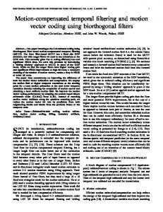
Fig. 1. Designation and location of spatial and temporal vectors used for the prediction. Fig. 2. Temporal DIRECT mode prediction for a B-slice. The current block is represented in black.

where is the motion vector and is the motion vector predictor (MVP). The MVP depends on the codec type. In hierarchical video coding [7], [8], each motion vector is predicted by the parent-node motion vector value. What is interesting in this method is the possibility to merge some nodes to reduce the number of motion vector residuals. As block coding schemes are included in the majority of standard video codecs, the MVP depends on the neighboring motion vectors in order to exploit spatial redundancies. Temporal redundancies have also been exploited as, for example, in [9], where good results in sequences with complex motion fields have been obtained. However, for sequences containing simple motion, using only the spatial predictor leads to better results. In [10], temporal and spatial correlations are exploited, however the choice between these correlations depends on local ad hoc statistics that does not ensure an optimal choice, contrary to the competition-based schemes. In [11], a selection between spatial and temporal predictors is made for the DIRECT mode only. In [12], three predictors are exhaustively compared, nevertheless, in this competition-based scheme, only spatial predictors are used, and, if a high difference in motion vector fields appears, temporal predictors are shown to be more efficient. B. MV Coding and Selection in H.264 H.264 is currently the most powerful video codec standard. This performance results from the new tools introduced for texture coding and the improvement of existing ones, as described in the introduction. Therefore, the motion information represents now an increased percentage of the bitstream and the efficient coding of this information becomes an essential objective. Two tools are implemented to this end: the MV prediction and the MV selection. 1) MV Prediction: H.264 applies predictive motion vector coding. The MVP in (1) is a median, for each component separately (horizontal and vertical), of the three neighboring motion vectors depicted in Fig. 1 ( , , and ). However, depending on the size of the current block, can be replaced by . In some particular cases, depending on the neighboring block properties, the value can be strictly equal to , , , or 0. These block properties depend on: the positions of the blocks , , , and (i.e., if these blocks belong to the image), the sizes of these blocks and of the current block, and on the reference frame used for each block prediction. In fact, if only one

of these motion vectors has the same reference frame as the current motion vector, the value will be equal to this vector. Note that, if the blocks , , , or are coded in intra mode (mode without motion vector), the value related to this block is considered to be 0. In video coding, a B-slice [13] is a slice that is encoded using past and/or future frames as references. The bidirectional prediction is a linear combination of two motion-compensated prediction signals that involve two motion vectors (one per motion-compensated prediction). Note that the reference frames for a bidirectional prediction can be a forward/backward pair, but also forward/forward and backward/backward pairs. The SKIP mode is a particular way of inter coding. A skipped macroblock has neither a block residue nor a motion vector or reference index parameter to transmit except the mode itself. Note that only one bit or less for 256 pixels will be transmitted in the bitstream. This mode is largely exploited, especially in sequences with static background. The motion predictor for this mode is equal to the value of the corresponding inter 16 16 except if or do not belong to the image or if the value of one of these vectors is null, when the predictor is equal to 0. As the SKIP mode for P-slices, B-slices have also a powerful prediction mode: the DIRECT mode [11]. It has two possible types: temporal and spatial, the type being fixed at each slice. The spatial DIRECT mode uses two spatial vectors. The temporal DIRECT mode uses the motion vector field of the future reference frame as depicted in Fig. 2. The two vectors for and ( designates the temporal DIRECT mode the predictors for the temporal DIRECT mode, while the suand refer to the lists of, respectively, past and perscripts future reference frames) are scaled according to the temporal distances between their respective reference and current frame. These motion vectors are defined by (2) (3) is the forward motion vector collocated in the fuwhere . is the temporal distance between ture reference frame the current frame and the past reference frame , and

Authorized licensed use limited to: Telecom ParisTech. Downloaded on January 6, 2009 at 04:54 from IEEE Xplore. Restrictions apply.

LAROCHE et al.: RD OPTIMIZED CODING FOR MOTION VECTOR PREDICTOR SELECTION

1249

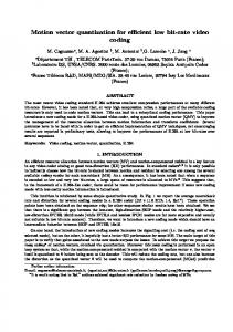
is the temporal distance between the forward and the backward reference P-frames. 2) MV Selection: The common aim of all video applications is the bitrate reduction with an increase in quality. This goal is achieved by minimizing the RD-criterion (4) where is the distortion and is the weighted rate corresponding to all the bitrate components [14] (5) where is the rate for block residue (luma+chroma), is the rate of the macroblock mode (SKIP or intra/inter prediction is the rate of the motion and macroblock partition type), is the rate of the others components: slice vector residue, and header, coded block pattern (CBP), stuffing bits, delta quantiza, , and are weighting factors depending on the tion. , quantization step. This weighted rate may be evaluated at different levels: sequence, slice, macroblock, and block, and therefore the competition may be applied at each one of these levels. The distortion is computed in the spatial or transformed domain and the rate components are estimated or really computed in exact number of bits depending on the application, as described in [2]. The JM H.264 reference software [3] is optimal in an RD sense but computationally intensive because this selection , process is made among all block partitions all reference frames, and at each subpixel accuracy. For the SKIP mode, the RD-criterion proposed in (4) yields (6) where is the distortion introduced by the SKIP mode. corresponds to the signaling of the SKIP Here, the term mode. Note that no one of the components entering , , or is necessary to be transmitted for the SKIP mode. In pracis negligible compared with the distortion tice, the cost and is often lower than one bit in both CABAC and CAVLC coding schemes. This means that, in the RD sense, it is more interesting to send nothing instead of the residual and the motion vector of an inter 16 16 macroblock. The evolutions of the bitrate proportions of the components in (5) depending on the quantization parameter are depicted in Fig. 3. One can remark is the major that, at a low bitrate, the motion information part of the total bitstream. Certainly, this figure shows these evolutions only for the Foreman CIF sequence for the High profile H.264, which is a sequence with complex motion fields, yet the motion information in other sequences can reach up to 38%. This large proportion proves the highest interest of the motion information cost reduction.

III. MV AND SKIP-MODE COMPETITION Here, we detail the two competition-based schemes for the prediction of the motion vectors for inter and for SKIP modes. The spatial, temporal and spatio-temporal sets of predictors are introduced, and then we discuss their adaptation to the case of multiple reference frames and of B-slices.

Fig. 3. Bitrate proportion depending on the quantization parameter using High IBBP profile H.264 for Foreman CIF sequence.

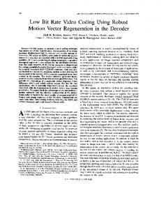
A. Competition-Based MV Coding 1) Predictor Set: The efficiency of a lossless coding method for the motion vectors is closely related to the predictors performance. The set can include several predictors, defined below, which are spatial, temporal, and spatio-temporal. The spatial predictors are the neighboring motion vec, , , , and the H.264 median predictor tors . We have also defined an extended spatial which is the median of , , and , for each component separately, if the blocks , , and belong to the image, if available, otherwise if available, otherwise returns if available or 0 value. The selection among the otherwise , , , or 0 does not depend on block sizes median or reference used. The temporal predictors are the collocated motion vector (motion vector at the same position in the previous which is the motion vector at the frame), the predictor position given by in the previous frame. The latter predictor has been defined to follow the motion of a moving , and ). object. Fig. 4 shows these vectors ( In this figure, all vectors point to the first previous frame. Fiand nally, two other temporal median predictors are defined by (7) (8) depicted in Fig. 1 are the neighboring where . motion vectors of Finally, spatio-temporal predictors are combinations of spais defined by tial and temporal ones. In particular, (9) Note that this weighted median prediction gives a higher imvalue than a simple median. As this set of portance to the predictors is relatively large, sometimes some of these predictors have the same value, yet each of them is relevant for specific contents and configurations. 2) Choices: In a competing scheme, two types of choices are possible.


1250


Fig. 4. Location of frame.

mv

,

mv

, and

mv

predictors for one reference

1) Adaptive choices: This choice is based on content or statistical criteria. Moreover, if the decoder is able to determine the mode, the index of the mode does not need to be transmitted which is an advantage for compression. 2) Exhaustive choices: All possible predictions are tested and therefore a mode needs to be transmitted in the bitstream. are With the use of choice 2), an index and a residual associated with each predictor (10) where is the number of predictors in the defined set. The index needs to be transmitted in the bitstream, and the weight of this new information is significant (on average, 3.5% of the bitrate and 12.5% of the motion information with only two predictors) [15]. As for all of the components of the bitrate, the cost of this new information must be introduced in the rate estimation. For the selection of the motion vector, the rate of the motion in (5) is replaced by to yield vector residue (11) contains the cost of the residual where cost of the index information

and the (12)

and

is the computed cost of the data

in the bitstream.

B. Competition-Based Skip Mode We have also introduced a competition-based scheme for the SKIP mode. This scheme uses several motion vectors as predictors leading to several SKIP modes. In this case, (6) is replaced by equations defined by (13) where and are the RD cost and the distortion re, is the set of motion vectors for the SKIP lated to is the number of predictors belonging to the mode, and set. Note that this scheme also involves the encoding of the index in the bitstream, except if all of the predictors are equal. Also, remark that we can use different predictors for motion compensation and for the SKIP mode, so in general .

Ref

Ref

Fig. 5. Motion vector collocated in pointing to and the current . The current block is represented in black. motion vector pointing to

mv

Ref

For competing coding, the use of adaptive choices has an interest for compression, because the index does not need to be transmitted. It seems interesting to combine the two choice types (exhaustive and adaptive). A set of relevant predictors in a given context could be defined by an adaptive method at sequence, scene, image, slice or block level. The main difficulty is to find statistical criteria allowing the best predictor choice. Then, the exhaustive choice is performed among this set of predictors. C. Multiple Reference Frames The multiple reference frames option uses several frames for motion compensation [16]. This option impacts the spatio-temporal correlations in the motion vector fields. Indeed, with this option, two neighboring motion vectors can relate to different reference frames. Thereby the temporal distances covered by these two vectors are different. This problem has been considacered in H.264 standard with the switch values of cording to reference frames used, as explained in Section II-B-I. The temporal correlation decreases when the distance between successive motion vector fields increases. An adaptation of the temporal predictors is therefore necessary to take into account the temporal distance between frames. We have thus added new sets, which use the refertemporal predictors in the and ence frame information. Following the assumption that an object moves with constant (the motion vector collocated in speed, the predictor pointing to the reference the previous reference frame ) is scaled according to the temporal disframe number , tances of the reference pictures used to the current block and the and , as depicted in Fig. 5. temporal distance between is the reference frame number pointed In this figure, by the motion vector of the current block. The scaled predictor is defined by (14) and and where is the temporal distance between is the temporal distance between the current frame and . This way of scaling the predictor is not the only possible solution to adapt temporal predictors according to the temporal



1251

distance. Another proposed predictor is the sum of temporally successive collocated vectors, described in the following. Let us consider that all motion vectors in each reference frame only point to their first previous frame (the temporal distance covered is by these vectors is equal to ). In this configuration, pointing to . the scaled motion vector collocated in is deThe sum of these successive temporal predictors fined by (15) where is the reference frame number of the current predictor block. The prediction efficiency of this vector is very close to , and therefore its cost in terms of rate would that of not justify to add a new predictor to the set of temporal predictors. In the same way, with the same configuration, we have con, a sum of predictors derived from the predictor sidered , defined by (16) where in is

is the motion vector at the position given by pointing to , except which

.

D. B-Slices For the B-slices, a competition between spatial and temporal DIRECT modes has been proposed in [11], where the competition is only for the DIRECT mode at different levels, such as slice or macroblock. Therefore, no modification of the DIRECT mode is proposed in this paper, and the MV resulting from the spatial DIRECT mode is not considered in our set of predictors. Moreover, in the H.264 standard, B-slices can be hierarchically ordered as defined in [17] (opposite to the classical successive order). For this particular ordering, an extended temporal DIRECT mode has been proposed in [18]. Let us introduce our motion vector competition for B-slices. The definition of efficient temporal predictors is related to the coding order and the number of B-slices between two P-frames. First, let us consider the case of successively coded B-frames. Generally, the motion vector field of one B-frame is related to the motion vector field of the forward reference frame because the motion vectors go through all B-frames and we suppose that an object moves with constant speed. This has already been exploited in the temporal DIRECT mode. So, the motion and devectors of the temporal DIRECT mode fined in (2) and (3) have been introduced in the set according to the coding mode of the future reference frames. We have also defined predictors based on the scheme of temporal DIRECT mode, in which the backward vectors are used. For this and , we have descheme, using the same convention for and given by fined (17) (18)

0

Fig. 6. Motion vectors collocated of the first previous B-frame B 1 with the associated temporal distances. The current block is represented in black.

where is the motion vector collocated in the past referis the frame which is pointed ence frame depicted in Fig. 2. and is the temporal distance between the past by and . reference frames The temporal redundancy between motion vector fields is clearly related to the temporal distance. The temporal distance is always higher than bebetween the current B-frame and tween the current and the previous B-frame, which is 1, except when the current frame is the last B-frame (B-frame number ). In this case, the two distances are equal. Moreover, the distance covered by a vector in a previous B-frame is lower than ; consequently, this vector is more accurate. each vector of We have thus created temporal predictors which use the motion (not available vector field of previously coded B-frame, -frame has for the first B-frame). A motion vector in the different possible directions (backward, forward, or backward and forward). According to these several cases, an adaptation and is defined. First, only the collocated motion of -frame pointing to a forward P-frame exists. vector in the , depicted in Fig. 6, is then used for the This vector scaling of the new predictors and defined by (19) (20) is the temporal distance between the forward where -frame. In the case of a backward block P-frame and the and residual prediction, we introduce the predictors as (21) (22) is the collocated motion vector in the where -frame pointing to the past P-frame, as depicted in Fig. 6. For and the forward and backward case, are available and thus is given by (19) and by (22). given by (21) and Note that, in this configuration, given by (20) can also be used.


1252


Note that, in the H.264 standard, a B-slice can use multiple forward and backward reference frames. The different schemes previously defined for P-slices in Section III-C can be used, especially the sum of scaled collocated motion vectors. For instance, the predictor for a motion vector related to forward , scaled to the first forward referP-frames is the sum of , where is the reference frame ence frame, and the used for block prediction. Here, we have described our competition-based scheme for the MV coding and the SKIP mode. Moreover, we have introduced several spatial, temporal, and spatio-temporal predictors with some scaling according to the multiple reference frames option and B-slices. These schemes have an impact on the complexity which is analyzed in Section IV. IV. COMPLEXITY ANALYSIS The proposed modifications are implemented in the JM10.0 H.264 reference software [3]. This C-code is neither optimized in terms of memory management nor in terms of computational efficiency. Therefore, it makes no sense to perform complexity measurements based on this software. We consequently find it more helpful and appropriate for future implementers to highlight the major impacts of the modifications on the algorithm and let them appreciate the impact on their own software or hardware platform. A. Memory Impact Using temporal predictors implies the storage of motion vectors and corresponding reference frame index. The size of this information depends on the search range, the number of reference frames, and the kind of temporal predictors used. These data are already stored for the B-slices by standard encoders and decoders supporting the Main and High profiles, given that similar data are needed to compute the temporal DIRECT mode. This additional memory requirement is consequently only for the Baseline profile and for the P-slices of the High profile. B. Computational Impact The computational impact on the encoder depends on the number and types of predictors used. First, each predictor needs to be computed based on the previously estimated motion vectors and using (7)–(9) and (14)–(22). Note that no new motion estimation needs to be performed compared with the H.264 is comreference. Then, for each predictor, the residual puted, and, in order to decide if the index needs to be sent or not, each predictor value is compared with all other predictor . It is important to notice that these values are the only mandatory impacts for the encoder to enable the competition. The other computations are non normative, and can be performed by different more or less complex means. In our implementation, the additional impacts are, for each predictor, given here: ; • the computation of the cost of the index , based • the computation of the cost of the residual on a look-up table corresponding to Exp-Golomb codes; • the computation of the distortion (SAD) for each predictor for the SKIP mode.

It is also expected that a realistic H.264 implementation has an early SKIP detection process [19] that allows checking first if the SKIP mode can be used, before testing all inter modes. In such a case, given that the number of macroblocks encoded in SKIP mode in our scheme is increased by 8.5%, some complexity savings can be expected. At the decoder side, the equality of the predictors needs to be checked both for the motion vector and SKIP modifications. This implies the computation of all predictors that belong to the . This only has an impact on the decoder. The sets and decoding of a skipped macroblock does not require the parsing of the bitstream (e.g., motion vector residue, reference frame, and block residue), inverse transform, or quantization. In [20], the time needed to encode and decode the VCEG test set when KTA tools are enabled in JM KTA 1.2 was provided. However, it was noted that this computational time does not fully reflect the real complexity of the tools. Since the C-code is not at all optimized, the complexity estimation based on the execution time tends to be largely overestimated. However, to give an idea, the computation time increase for our proposed scheme with two predictors for the motion vector prediction and SKIP mode is about 7% at the encoder side and 4% at the decoder side. With our modifications the number of skipped macroblocks is increased and thus it is highly expected that the computational complexity of the decoder decreases in a realistic implementation. In the light of these remarks we believe that the average complexity increase remains low and more than acceptable for both profiles, especially when considering the tradeoff with the quality improvements which are detailed in Section V. V. EXPERIMENTAL RESULTS A. Test Conditions Simulations were performed on the JM10.0 H.264 reference software [3] in which all normative tools and efficient nonnormative encoding decisions are implemented. Two profiles are selected: Baseline and High. The High profile corresponds to the highest possible quality using all H.264 normative tools such as B-slices, CABAC entropy coding, and 8 8 transform. The Baseline profile has been created for mobile applications, with a lower complexity than the High profile: only I- and P-slices and the CAVLC entropy coding are used. For these two profiles, as recommended in [21], we selected a 32 32 search range, . four reference frames, and RD-optimization With RD-optimization option, each rate in (5), (6), (12), and (13) of each coding mode is computed in exact number of bits by CAVLC or CABAC, depending on the chosen profile. For the High profile, we have selected the High IBBP configuration which used two successive B-frames between two P- (or I- at the beginning) frames. The test set is composed of 9 CIF, 4 SD, and 2 sequences 720 p of 100 frames each, with various representative contents and motions. Quantization parameters are equal to 28, 32, 36, and 40. For these QPs, the quality is between 28 and 40 dB which corresponds to a visual quality in line with most of the industrial applications. All of the results in this section are given in percentage of bitrate savings computed with the recommended VCEG metric



1253

TABLE I PERCENTAGE OF THE SELECTION OF EACH PROPOSED PREDICTOR FOR MOTION VECTOR COMPETITION FOR THE CIF TEST SET SEQUENCES IN THE BASELINE PROFILE

TABLE II MOTION VECTOR COMPETITION IN THE BASELINE PROFILE: BITRATE SAVINGS FOR DIFFERENT PAIRS OF PREDICTORS

defined in [22], which is an average PSNR difference between two RD-curves computed with the difference between the integrals divided by the integration interval. This metric was preferred to a classical computation of PSNR since it integrates in a single figure a simultaneous difference in PSNR and bitrate.

TABLE III GLOBAL BITRATE SAVINGS FOR EACH SET COMBINATION OF MOTION VECTOR COMPETITION AND SKIP-MODE COMPETITION. AVERAGE GAIN COMPUTED FOR THE SET OF ALL CIF SEQUENCES

B. Baseline Profile 1) Predictor Sets: The efficiency of the proposed competition schemes depend on the number and type of predictors. We have performed extensive experiments to find the best configuration. First, in order to motivate the choice of the proposed predictors, we have examined the percentage of selection of each of the proposed predictors over the entire test set by including the 11 predictors in the set . Table I illustrates the fact that, in different configurations and for different contents, each predictor may be optimal in an RD sense and shows the interest of considering these predictors for further investigation. In order to select the best configuration for the motion vector competition, we have compared several sets containing two predictors. Table II represents the bitrate savings, for all CIF seis combined one by one with each prequences, where dictor described in Section III. The best average bitrate saving and the scaled colloresults from the combination of . Moreover it can be remarked that the cated vector average bitrate saving is higher with the combination of the and a temporal predictor than for with a spatial predictor. For the SKIP mode competition a similar experiment has been made and the results prove that the combination of two spatial predictors gives better results. These two sets provide the best average result on the selected test set, yet not the best result for each sequence. For instance, having two spatial predictors is better suited for very fast motion sequences. The next experiments aim at selecting the optimal number of predictors in the sets. We have tested with either one, two, and four predictors for motion vector competition and for the SKIP mode competition. The best tradeoff is obtained with two predictors for motion vectors and two predictors for SKIP mode as shown in Table III, where global bitrate savings are reported. , The sets of motion vector predictors are (the best combination from . Table II) and sets for motion vector SKIP mode are, respecThe , , and tively,

. It can be noticed that, except for a minority of sequences, the bitrate reduction for the configuration with two predictors for motion vector and SKIP mode is higher. Obviously, the reduction of the is increased when using four premotion vector bitrate dictors, but the compromise with the index coding leads to slightly worse results. In the same way, when using four predictors for SKIP, the number of SKIP increases but the distortion introduced is higher than with two predictors. Again, an adaptive set of predictors according to statistical and local characteristics is expected to increase the gain. 2) Predictor Selection For MV Competition: For motion vector competition, the analysis of the selection of the spatial or temporal prediction has been performed and the results are provided in Table IV. It shows that on average on the test is selected 44% of the set, the temporal predictor time. Given that the selection results from an RD choice, this average result confirms that the temporal predictors are useful. Note that these values exclude the cases where both predictors provide the same value, which represents 11% in average. As an interesting feature, the percentage of selection of the temporal predictor increases when the QP increases. A reason for this is that with larger QP (lower bitrate), the percentage selection of the 16 16 prediction mode increases, and thus the spatial correlation between neighboring motion vectors decreases, while the correlation with the collocated vector remains the same. Sequence by sequence the percentage of temporal predictor selection varies between 26% and 60% depending on the sequence type. For sequences with static background, such as Ice


1254


TABLE IV DISTRIBUTION OF THE PREDICTOR SELECTION (BASELINE PROFILE)

TABLE V DISTRIBUTION OF THE PREDICTOR SELECTION FOR EACH REFERENCE FRAME Ref IN THE BASELINE PROFILE (ONLY PAST FRAMES, ORDERED BY INCREASING TEMPORAL DISTANCE TO THE CURRENT FRAME). AVERAGE OCCURRENCE COMPUTED ONLY FOR CIF SEQUENCES

and Mobile, the temporal predictor is more often selected than for sequences with a global motion. The temporal selection is also correlated with the reference frame used for block prediction of the current block. Table V shows the percentage selection of and and when these two predictors have the same value according to each reference frame. The temporal predictor selection increases with the temporal distance to the reference frames, which may appear strange at first sight. This selection is higher starting from the second reference frame. This increase proves the interest of the predictor adaptation according to the temporal distance between motion vector fields. Indeed the selection of the further reference frames also increases. For CIF sequences, the fourth reference frame selection is increased by 38% com. However, note that, in all pared to the simple use of cases, the predictor is obtained by scaling the collocated vector on the previous frame which does not depend on the distance between the current frame and the reference frame. 3) SKIP-Mode Competition: Fig. 7 shows the percentage of increase of the number of macroblocks encoded with the SKIP mode. The average is 8.5%. This increase is correlated with the QP and with the sequence type. For sequences with large objects and fluid motion like Soccer or Crew, the percentage of SKIP selection is increased using the proposed scheme. However, we can notice that selecting a spatial predictor as the second predictor is less efficient for sequences with static background such as BBC news and Modo or Ice and Mobile. Such sequences benefit more from a configuration with one spatial and one temporal predictor. For instance, the percentage bitrate savings obtained and in the set is 6.7% on BBC news with against 5.8% for the proposed scheme. As in this section we have illustrated the combination of a competing scheme on motion vector predictors and a competing

Fig. 7. Percentage increase of skipped macroblocks, for each sequence, at each QP value.

scheme on the SKIP mode, it is interesting to note the individual gain related to each scheme. As illustrated in Table III, the average bitrate gain resulting from the competition-based SKIP mode alone is 2.6% (second line), and the savings resulting from the modification on the motion vector coding leads to an average bitrate gain of 3.5% (third line). Moreover, as it can be seen from the fourth line of Table III, the global bitrate savings obtained by combining the best sets of predictors is almost the sum of these individual increases (5.9%). This result proves the complementarity of the two schemes. Indeed, only with the competition-based SKIP modes, the number of bits per vector increases and only with the modification on motion vector, the number of SKIP mode decreases, while with the combination of these two methods, none of the inter modes is penalized. 4) Global Bitrate Reduction On the Test Set: Table VI presents the percentage of bitrate saved for each sequence using the competition for both motion vector prediction and the SKIP mode. It can be noticed that the proposed method offers a compression gain for all sequences of the test set. Of course, this test set is composed of sequences with motion and some of them with complex or fast motions, which implies a large proportion of motion information in the bitstream. Nevertheless, compression gains are also obtained on sequences with simple or no motion (e.g., videoconferencing sequences) such as Paris and Akiyo. These gains are, respectively, 3.2% and 3.9%. For this kind of sequences, the SKIP mode is already widely used, and consequently the increase of number of SKIP mode is lower and the proportion of motion information is already low. For sequences with fast or complex motions, the compression gain is higher and sequences exhibiting global and constant motion, combined with a high level of spatial details (such as City) take full advantage of the temporal prediction, whereas the classical spatial median usually fails. The increase of bitrate reduction is also closely related to the increase of distortion, as depicted in Fig. 8. These results are computed as described in [23]. The RD curves for the same sequences are presented in Fig. 9, illustrating the efficiency of the method across different rate points. At low bitrates, the motion information tends to become a significant part of the total bitstream, so its reduction leads to the highest improvements. Finally, the birate reduction is not related to the resolution, yet clearly to the frame rate. For instance, the bitrate saving for Foreman at 30 Hz is 7.7% and for the same sequence at 15 Hz the bitrate saving is 4.1%.



1255

TABLE VI GLOBAL AVERAGE BITRATE REDUCTION FOR EACH SEQUENCE IN THE BASELINE PROFILE USING BOTH MV AND SKIP-MODE COMPETITION

Fig. 8. Percentage global bitrate reduction compared with H.264 Baseline for four sequences.

TABLE VII BITRATE SAVINGS ON P-FRAMES ACCORDING TO EACH COMBINATION OF MOTION VECTOR AND SKIP-MODE PREDICTORS IN THE HIGH IBBP PROFILE. AVERAGE GAIN COMPUTED ONLY FOR CIF SEQUENCES

Fig. 9. RD curves of four sequences compared with H.264 Baseline profile.

This is explained by the temporal distance between the motion vector fields. With a frame rate equal to 15 Hz, the temporal distance is larger and the efficiency of the collocated motion vector is lower. Finally, the average bitrate gain is 7.7% and reaches 45% for the Raven sequence at QP 40 (to be precise, a simultaneous gain of 38% in bitrate in addition to a gain of 0.3 dB). C. High Profile In this profile, the problem is slightly modified due to the presence of B pictures, where B stands for bipredictive (and not

necessarily bidirectional) and multiple reference frames, which allow new choices for the selection of the predictors. The related questions to be answered are the following. • Is the set used for the P-frames in the Baseline profile still adapted to the High profile, where the temporal distance between P-frames is increased? • Which set is the most adapted to the B-frames, and is it the same for all the B-frames between two P-frames? Table VII gives the average birate savings on P-frames for sets. The same sets as the several combinations of and ones proposed for the Baseline profile give the best results for the P-frames. Most remarks made for the experimental results in the previous section are still true, such as the frame rate or the temporal distance between two motion vector fields influence on the efficiency of temporal predictors and the selection of the temporal predictor increases with QP values and furthest reference frames. Now the temporal distance between two P-frames is larger and, consequently, the temporal correlation between motion vector fields is smaller. As depicted in Table IX, the average selection of the temporal predictor is 26% against 44% in Baseline profile (Table IV). This decrease yields a reduced gain on P-frames (2.5%) compared to the gain on P-frames for the Baseline profile (6.5%). The reduced gain on P-frames is partly compensated by the gain on B-frames. The efficiency of predictors varies with the number of B-frames used. As for the P-frames, the combination of one spatial and one temporal predictor gives the best


1256


TABLE VIII BITRATE SAVINGS ON THE FIRST AND SECOND B-FRAMES DEPENDING ON THE PROPOSED PREDICTORS. AVERAGE GAIN COMPUTED ONLY FOR CIF SEQUENCES

TABLE X AVERAGE GLOBAL BITRATE REDUCTION FOR EACH SEQUENCE IN THE HIGH IBBP PROFILE USING BOTH MV AND SKIP-MODE COMPETITION

TABLE IX DISTRIBUTION OF THE PREDICTOR SELECTION IN THE HIGH IBBP PROFILE FOR THE P- AND B-FRAMES

results. The spatial predictor selected is . Table VIII illustrates the average gain on each B-frame ( , ) related to the second temporal predictors. In this table, is the motion vector collocated in the future frame without scaling. The represents the scaled predictors collocated in the represents the past frame given by (17) and (18). The scaled predictors collocated in the frame given by (2) and (3). The represents the scaled predictors collocated in the -frame given by (19)–(22) according to the directions and the availabilities of the collocated vectors. Finally, after sevfor frame which leads eral tests, we have defined the to the best results. This predictor is equal to value if the collocated block is not intra coded, else this predictor is equal to the value. The interest of the motion vector scaling is still showed with the increase of bitrate for . Then, the difference of bitrate saving for and proves that the motion vector field of a B-frame is more correlated with the future reference frame, which goes through all B-frames, than with the past are reference frame. Finally, the best second predictors for given by because and predictors cover a smaller distance than which gives higher precision. This predictor generates a higher bitrate saving percentage on than on the first B-frame which can only use . In the sequel of this section the experimental results are given with this configuration. Table IX shows the average percentage selection of each predictor for P, first, and second B-frames on the whole test set. For - and -frames, the temporal predictors proposed are more often selected than the classical . It can be noticed that this selection is slightly higher for the second B-frame. This still proves the highest importance of the temporal distance between motion vector fields.8 Finally, Table X presents the percentage of bitrate saved for each sequence. As in the experimental results described for the Baseline profile, our method offers a compression gain for all sequences of the test set. The average bitrate saving for the High

profile is 4.3%. This lower gain than for the Baseline profile is explained by the results obtained on P-frames, which represent in average 65% of the global bitrate with two B-frames configuration. VI. CONCLUSION In this paper, two competition-based schemes are proposed, one for the prediction of the motion vectors and one for the SKIP mode. The motion vector predictions are selected via an RD-criterion that considers the cost of the residual and the index for the prediction. The same scheme is applied to select the best predictor for the SKIP mode. Temporal and spatial predictors are thus added to the standard motion vector predictor with the aim to exploit both temporal and spatial correlations between the motion vector fields. Moreover, the use of multiple reference frames and B-slices gives rise to some adaptations of predictors. Thereby, in this paper, some scaled temporal predictors have been proposed according to the temporal distance between the motion vector fields. These two combined techniques, implemented in the JM10.0 H.264 reference software for Baseline and High profile, provide a systematic bitrate reduction (computed with the VCEG metric) with a decrease of the computational complexity at the decoder. For the recommended VCEG configurations in the Baseline and the High profile, the average bitrate savings are, respectively, 7.7% and 4.3%. The gain can reach up to 45% on one sequence 720 p at 60-Hz frame rate for Baseline profile. These gains are obtained with the use of a spatial and a temporal predictor for the competition-based scheme on motion vectors and with two spatial vectors for the SKIP-mode modification. However, other predictor combinations give some interesting results on specific sequences or QPs. An adaptation of predictors set according to the statistical characteristics of the sequence should allow to increase even more the bitrate saving.



REFERENCES [1] Advanced Video Coding for Generic Audiovisual Services, ITU-T Recommendation H.264 and ISO/IEC 14496–10 AVC Std., , 2005, Rev. version 3. [2] K. P. Lim, G. J. Sullivan, and T. Wiegand, “Text description of JM reference encoding methods and decoding concealment methods,” JVT of ISO/IEC MPEG and ITU-T VCEG, Hong-Kong, 2005, Draft of Joint Model JVT-N046. [3] K. Suehring, “H.264/AVC Software Coordination” [Online]. Available: http://iphome.hhi.de/suehring/tml/ [4] T. Wedi, 1=8-Pel Motion Vector Resolution for H.26L ITU-T VCEG, Portland, USA, 2000, Proposal Q15-K-21. [5] J. Jung and G. Laroche, “Competition-based scheme for motion vector selection and coding” ITU-T VCEG, Klagenfurt, Austria, 2006, Information VCEG-AC06. [6] L. A. S. C. Da and J. W. Woods, “Adaptive motion vector quantization for video coding,” in Proc. IEEE ICIP, Oct. 2000, vol. 2, pp. 867–870. [7] A. Deever and S. S. Hemami, “Dense motion field reduction for motion estimation,” Signals, Syst. Comput., vol. 2, pp. 944–948, Nov. 1998. [8] M. H. Chan, Y. B. Yu, and A. G. Constantinides, “Variable size block matching motion compensation with applications to video coding,” in Proc. Inst Elec. Eng., Aug. 1990, vol. 137, pp. 205–212. [9] J. Yeh, M. Vetterli, and M. Khansari, “Motion compensation of motion vectors,” in Proc. IEEE ICIP, Oct. 1995, vol. 1, pp. 574–577. [10] M. C. Chen and A. N. Willson, “A spatial and temporal motion vector coding algorithm for low-bit-rate video coding,” in Proc. IEEE ICIP, Oct. 1997, vol. 2, pp. 791–794. [11] A. M. Tourapis, F. Wu, and S. Li, “Direct mode coding for bipredictive slices in the H.264 standard,” IEEE Trans. Circuits Syst. Video Technol, vol. 15, no. 1, pp. 119–126, Jan. 2005. [12] S. D. Kim and J. B. Ra, “An efficient motion vector coding scheme based on minimum bitrate prediction,” IEEE Trans. Image Process., vol. 8, no. 8, pp. 1117–1120, Aug. 1999. [13] M. Flierl and B. Girod, “Generalized B pictures and the draft H.264/AVC video-compression standard,” IEEE Trans. Circuits Syst. Video Technol., vol. 13, no. 7, pp. 587–597, Jul. 2003. [14] G. J. Sullivan and T. Wiegand, “Rate-distortion optimization for video compression,” IEEE Signal Processing Mag., pp. 74–90, 1998. [15] G. Laroche, J. Jung, and B. Pesquet-Popescu, “A spatio-temporal competing scheme for the rate-distortion optimized selection and coding of motion vectors,” in Proc. Eur. Signal Processing Conf., Florence, Italy, Sep. 2006. [16] T. Wiegand, X. Zhang, and B. Girod, “Long-term memory motioncompensated prediction,” IEEE Trans. Circuits Syst. Video Technol, vol. 9, no. 2, pp. 70–84, Feb. 1999. [17] H. Schwarz, D. Marpe, and T. Wiegand, Hierarchical B Pictures JVT of ISO/IEC MPEG and ITU-T VCEG, Poznan, Poland, 2005, Information JVT-P014. [18] D. Zhao, W. Gao, Q. Huang, S. Ma, and Y. Lu, “New bi-prediction techniques for B pictures coding,” in Proc. IEEE ICME, 2004, vol. 1, pp. 101–104. [19] B. Jeon, Fast Mode Decision for H.264 JVT, Waikoloa, HI, 2003, Proposal JVT-J033. [20] J. Jung and G. Laroche, Performance Evaluation of the KTA 1.2 Software ITU-T VCEG, Marrakech, Morocco, 2007, Information VCEGAE09. [21] T. K. Tan, G. J. Sullivan, and T. Wedi, “Recommended simulation common conditions for coding efficiency experiments” ITU-T VCEG, Nice, France, 2007, Input/Discussion VCEG-AE10.

1257

[22] Calculation of Average PSNR Differences Between RD-Curves ITU-T VCEG, 2001, Proposal VCEG-M33. [23] J. Jung and S. Pateux, An Excel Add-in for Computing Bjontegaard Metric and its Evolution ITU-T VCEG, Marrakech, Morocco, 2007, Information VCEG-AE07.

Guillaume Laroche received the M.S. degree in image processing from Rene Descartes University, Paris V, Paris, France, in 2005. He is currently working toward the Ph.D. degree at France Telecom R&D and Ecole Nationale Superieure des Telecommunications, Paris. His current research interests are video-coding with competitive schemes.

Joel Jung received the Ph.D. degree from the University of Nice-Sophia Antipolis, Nice, France, in 2000. From 1996 to 2000, he was with the I3S/CNRS Laboratory, University of Nice-Sophia Antipolis, where he was involved with the improvement of video decoders based on the correction of compression and transmission artifacts. He joined Philips Research France in 2000 as a Research Scientist in video coding, postprocessing, perceptual models, objective quality metrics, and low-power codecs. He is currently with France Telecom R&D Labs, Paris. He is an active participant in standardization for video compression with more than 20 contributions to the Video Coding Expert Group ITU-T SG16-Q6. He holds 25 patents in the field of video coding.

Beatrice Pesquet-Popescu (SM’06) received the engineering degree in telecommunications from the “Politehnica” Institute, Bucharest, Romania, in 1995, the Ph.D. degree (with honors) from the Ecole Normale Suprieure de Cachan in 1998, and the “Habilitation Diriger des Recherches” from the Ecole Nationale Superieure des Telecommunications (ENST), Paris, France, in 2005. In 1998, she was a Research and Teaching Assistant with Universit Paris XI, and in 1999 she joined Philips Research France, where for two years she was a Research Scientist and then Project Leader, involved with scalable video coding. Since October 2000, she has been an Associate Professor in multimedia with ENST. Her current research interests are in scalable and robust video coding, adaptive wavelets and multimedia applications. Dr. Pesquet-Popescu is an EURASIP AdCom member, a member of the Administrative Committee of the French GRETSI Society and an IEEE Signal Processing Society MMSP Technical Committee. She was a recipient of the Best Student Paper Award in the IEEE Signal Processing Workshop on Higher-Order Statistics in 1997, the Bronze Inventor Medal from Philips Research, and in 1998 she received a Young Investigator Award from the French Physical Society.
