Interactive Display of Surfaces Using Subdivision ... - CiteSeerX

Interactive Display of Surfaces Using Subdivision Surfaces and Wavelets Mark A. Duchaineau, Lawrence Livermore National Laboratory Martin Bertram, University of Kaiserslautern Serban Porumbescu, CIPIC, University of California, Davis Bernd Hamann, CIPIC, University of California, Davis Kenneth I. Joy, CIPIC, University of California, Davis

Abstract Complex surfaces and solids are produced by large-scale modeling and simulation activities in a variety of disciplines. Productive interaction with these simulations requires that these surfaces or solids be viewable at interactive rates – yet many of these surfaces/solids can contain hundreds of millions of polygons/polyhedra. Interactive display of these objects requires compression techniques to minimize storage, and fast view-dependent triangulation techniques to drive the graphics hardware. In this paper, we review recent advances in subdivision-surface wavelet compression and optimization that can be used to provide a framework for both compression and triangulation. These techniques can be used to produce suitable approximations of complex surfaces of arbitrary topology, and can be used to determine suitable triangulations for display. The techniques can be used in a variety of applications in computer graphics, computer animation and visualization. Keywords: subdivision surfaces, wavelets, isosurfaces, visualization

1

Introduction

The advent of high-performance computing has completely transformed the nature of most scientific and engineering disciplines, making the study of complex problems from experimental and theoretical disciplines computationally feasible. All science and engineering disciplines are facing the same problem: How to archive, transmit, visualize, and explore the massive data sets resulting from modern computing, Today, when only small amounts of data must be processed, many researchers can accomplish some of these objectives on a desktop machine. But the “impact problems” of science and engineering typically require the analysis of data sets that need massive storage capability and large-scale display hardware for visualization. The exploration of truly massive data sets requires new techniques in compression, storage, transmission, retrieval, and visualization, as the existing techniques

for small data sets do not scale well, or not at all. A new approach is needed to address the interrelated problems of storage, visualization, and exploration of these massive data sets. Traditionally, due to smaller and simpler data sets to be studied, researchers have developed “in-core” visualization and data exploration methods that work well on small or medium-scale data sets. But today’s scientific and engineering problems require a different approach to address the massive data problems in organization, storage, transmission, visualization, exploration, and analysis. Terascale physics simulations are now producing tens of terabytes of output for a several-day run on the largest computer systems. An example is the Gordon Bell Prizewinning simulation of a Richtmyer-Meshkov instability in a shock-tube experiment [46], which produced isosurfaces of the mixing interface with 460 million unstructured triangles using conventional extraction methods. Similarly, the Digital Michelangelo Project [38] is generating data sets with 500 million data points, and in both problem areas, billion-triangle surfaces are expected shortly. In the Gordon Bell isosurface case, if we use 32-bit values for coordinates, normals and indices, then we require 16 gigabytes for the storage of a single isosurface, and several terabytes for a single surface tracking through all 274 time steps of the simulation. With the gigabyte-per-second read rates of current RAID storage, it would take 16 seconds to read a single surface. Another bottleneck occurs with high-performance graphics hardware. Today, the fastest commercial systems can effectively draw around 20 million triangles per second, i.e. around 1 million triangles per frame at 20 frames per second. To achieve interactive rates, a terabyte data set requires almost a thousand-fold reduction in the triangle count. Wavelet compression and view-dependent optimization are two powerful tools that we use to reduce the size of these data sets. Conversion is required to turn irregular extracted surfaces into a form appropriate for these algorithms (see Figure 1). Section 2 discusses a novel lifting procedure that generates subdivision-surface wavelets for Catmull-Clark sub-

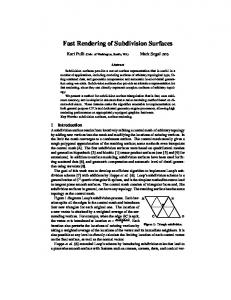
Figure 1: Shrink wrapping steps (left to right): the full-resolution isosurface, the base mesh constructed from edge collapses, and the final shrink-wrap with subdivision-surface connectivity. v

division surfaces. Section 3 discusses the use of these wavelets to generate approximations to isosurfaces. We discuss the fitting methods in Section 4, and the remapping procedure that obtains better parameterizations of the surfaces in Section 5. The results of our method are shown in Section 6.

v

v e ve

vf f v

v

f f

f

2

Bicubic Subdivision-Surface Wavelets

Subdivision surfaces are limit surfaces that result from recursive refinement of polygonal base meshes. A subdivision step refines a submesh to a supermesh by inserting vertices. The positions of all vertices of the supermesh are computed from the positions of the vertices in the submesh, based on certain subdivision rules. Most subdivision schemes converge rapidly to a continuous limit surface, and a mesh obtained from just a few subdivisions is often a good approximation for surface rendering. Subdivision surfaces that reproduce piecewise polynomial patches can be evaluated in a closed form at arbitrary parameter values [56]. There exists a variety of different mesh-subdivision schemes. We utilize Catmull-Clark subdivision [7], which generalizes bicubic B-spline subdivision to arbitrary topology. In this scheme, vertices in the supermesh correspond to faces, edges, or vertices in the submesh. In the following, we denote the corresponding vertex types as , , and , respectively. All faces produced by Catmull-Clark subdivision are quadrilaterals. For our wavelet construction, we use the Catmull-Clark subdivision structure with slightly different subdivision rules. To describe subdivision rules that determine new vertex positions, we use an index-free notation. We use the averaging operator x y , where x and y can represent , , or . This operator returns for every vertex of type y the arithmetic average of all adjacent vertices of type x. If there are no direct neighbors of type x, then x y returns

fe

v

e

v v

v

f

vv

v

fv

v f

v

f fe

v

v v

e

f

f f

v

v f

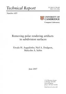
Figure 2: Examples for index-free notation. The point f is the centroid of a face; e is the midpoint of an edge; e is the midpoint of the line segment defined by vertices; v is the centroid of all adjacent vertices; and v is the centroid of vertices.

v

v

f

v

f

f

the average from those vertices of type x that correspond to adjacent primitives, i.e., adjacent vertices or incident edges or faces. Examples for the averaging operator are shown in Figure 2. To provide an example of the index-free notation, we formulate the Catmull-Clark subdivision rules in algorithmic notation using the x y operator:

1 f 2 e 3 v

vf

:

v + f e
f + vv + (

1 e 2 1 v nv

:

:

nv

2)v




(1)

Here, nv denotes the valence of a vertex. The three rules are illustrated in Figure 3. The vertices are initially defined by the coordinates given by a submesh. The first rule defines each vertex to be located at the centroid of its corresponding face. The second rule defines each vertex to be the average of its edge midpoint v and the midpoint e of the two adjacent vertices. The third rule re-defines the position for each vertex as a weighted sum of its neigh-

v

f

v

f

v

e

f

v

v

v f

f

v

v

f

f

e

f f

f v

v

v

v

v f

v

v

Figure 3: Catmull-Clark subdivision rules (apply left to right)

e’

e

Figure 5: Lifted cubic B-spline wavelet.

v’

v

Figure 4: Wavelet decomposition coarsens a control polygon and stores difference vectors in place of removed vertices.

f

v

boring vertices, its adjacent submesh vertices v , and its own location. This vertex-modification step is performed simultaneously for all vertices. Subdivision rules like these define vertex modifications that are necessary to determine all supermesh coordinates for an individual subdivision step. For the next subdivision step, all vertices become vertices again, and the same subdivision rules are applied recursively.

v

2.1

To obtain a smooth approximating curve, the reconstruction process can be terminated at any level of resolution providing a control polygon at an intermediate level of detail. The curve is obtained by applying the subdivision operator ad infinitum and assuming zero detail on all finer levels. In the case of B-spline wavelets, the operator reproduces in the limit a B-spline curve with uniform knot vector. A B-spline curve can be computed directly from a control polygon [23]. The reconstruction rules for a cubic B-spline wavelet transform can be defined in index-free notation as follows:

S

S

1 v 2 e 3 v : :

:

Lifted One-Dimensional Wavelets

Decomposition rules for a DWT are defined by two linear operators, a fitting operator predicting the vertex coordinates for the coarser polygon, and a compaction-ofdifference operator representing the reduced details:

F

C v0 = F(v e) and e0 = C(v e) ;

;

(2)

:

Decomposition is recursively applied to a coarse polygon until a base resolution is reached. A DWT thus provides a base polygon and all individual levels of detail that need to be added recursively to reconstruct an original polygon. An inverse DWT is defined by reconstruction or synthesis rules that invert the decomposition rules. Starting with a base polygon, an inverse DWT applies reconstruction rules recursively in reverse order of decomposition and thus adds more and more detail to a polygon. Reconstruction rules are defined by a subdivision operator predicting the shape of a next finer control polygon and an expansion operator providing the missing details:

S

E

 

v = S(v0 ) + E(e0) e

:

(3)

v 34 ev e + ve 1v + 1e 2 2 v

(4)

These three vertex modifications represent lifting operations for the DWT. Lifting is used to define the shape of wavelets with certain properties, like vanishing moments. The subdivision operator is obtained from these reconstruction rules by assuming zero wavelet coefficients 0 . Vertices of type 0 and 0 represent coefficients for wavelets and B-spline scaling functions, respectively. A cubic B-spline wavelet obtained from our construction is depicted in Figure 5. To construct the corresponding decomposition rules we invert the three individual lifting operations in reverse order. The decomposition rules are defined as:

S

e

e

1 v 2 e 3 v :

:

:

2.2

v

2v ev e ve v + 34 ev

(5)

Wavelets on Polygon Meshes

In the special case of a rectilinear mesh, a tensor-product DWT is defined by performing a one-dimensional DWT for all rows and then for all columns of the mesh. The corresponding tensor-product approach for the first lifting

e

f

v

e

e

f

This reconstruction formula defines linear subdivision and expansion operators, given by

f

f

e

f

e

e

v

e

0 1

f

@ A

f

f

e

v e = S(v0 ) + E(e0 f 0 ) f

Figure 6: Tensor-product lifting operation on a rectilinear grid. A one-dimensional lifting operation is applied first to the rows and then to the columns of a grid. e

f

f

f

e

f v

e

v e

f

e

e

f

f

e e

e

1 2 3 4 5 6

:

Figure 7: Same tensor-product lifting operation as in Figure 6, applied to arbitrary polygonal meshes.

:

: :

operation of the reconstruction rules (4),

v

:

e

(6)

is illustrated in Figure 6. We note that the tensor-product lifting scheme also involves vertices and that vertices act like vertices for exactly one direction. The fundamental observation that makes our lifting approach possible is that this tensor-product lifting operation can be computed by modifying vertices and vertices separately, see Figure 7. This formulation does not require vertex valences to be four, and it is thus applicable to arbitrary polygonal base meshes. A generalized tensorproduct lifting operation for equation (6) is defined by the rules

f

v

e

e

e v

e v

f

3 4 e 9 16 v

f

e

(7)

Due to the averaging operators, the total weight added to an individual vertex remains independent of its valence. This property ensures that the shapes of basis functions near extraordinary points are close to the shapes of corresponding basis functions on regular domains. Analogously to the first reconstruction rule in (4) the two remaining rules can be generalized to arbitrary polygonal meshes. This is the entire set of reconstruction rules for the lifted generalized bicubic DWT:

1 2 3 4 5 6

: :

: :

:

:

e v e f e v

e 34 f e v 169 f v 32 ev e + ve f vf + 2ef 1 1 2e + 2fe 1f + e 1v v 4 4 v :

4v + f v 4ev 2e f e f + vf 2ef e ve v + 169 f v + 32 ev e + 34 f e

v0 = F(v e f) and e = C(v e f) f0

 0

(10)

;

;

;

;

(11)

:

Our DWT is now applied as follows: a polygonal base mesh defining a surface topology is recursively subdivided using Catmull-Clark subdivision structure until a prescribed resolution is obtained. A mapping between the fine mesh and the geometry that needs to be represented is established. Coordinates for each mesh vertex are estimated so that the fine mesh (and the limit surface obtained by ) approximates the geometry closely. The actual input for our DWT is a hierarchical mesh structure with associated vertex coordinates at the finest subdivision level. Decomposition rules (10) are applied recursively from fine to coarse until the base mesh is obtained. The latter now contains control points for the geometry at coarsest resolution. The wavelet coefficients corresponding to vertices on any finer subdivision level contain surface details. A control mesh represents, at any resolution, a smooth generalized bicubic B-spline surface.

S

2.3 (8)

v e f e v e

In analogy to equation (2), these decomposition rules define linear fitting and compaction-of-difference operators, given by

v

3 2 v

S

f

:

v

(9)

:

On a rectilinear grid, the subdivision operator reproduces bicubic B-splines (scaling functions) as limit surfaces when no detail is added, i.e., when all wavelet coefficients 0 and 0 are zero. On arbitrary polygonal base meshes, the subdivision scheme behaves similar to Catmull-Clark subdivision. The corresponding decomposition rules are defined by inverting the rules (8) in reverse order:

f

3 4 v

;

Boundary Curves and Feature Lines

Boundary curves and sharp feature lines need to be treated differently in the wavelet scheme in order to avoid a large number of non-zero wavelet coefficients and to predict coarser levels of resolution more precisely. Feature lines for subdivision surfaces were described for by by DeRose et al.[14]. Boundaries and features correspond to marked

edges in the base-mesh that are subdivided like B-spline curves defined by - and vertices. It is also possible to define sharp vertices that cannot be modified by any subdivision rule. (To improve the surface quality in the neighborhood of sharp vertices, adjacent edges are treated like sharp edges.) To handle sharp edges and vertices correctly, our subdivision operator must apply one-dimensional subdivision rules for all and vertices belonging to sharp edges and it must not modify sharp vertices. Therefore, our reconstruction rules (8) need to be modified in the following way:

v

S

v

  

(2 + 1) (2 + 1)

e

Signed distance transform: for each grid point in the 3D mesh, compute the signed-distance field, i.e. the distance to the closest surface point, negated if in the region of scalar field less than the isolevel. Starting with the vertices of the 3D mesh elements containing the isosurface, the transform is computed using a breadth-first propagation.

e

For any vertex located on a sharp edge or belonging to an edge with a sharp vertex, the first and fifth rules are ignored. For any sharp ignored.

v vertex, the second and sixth rules are

v

For any vertex that has incident sharp edges and that is not sharp itself, the second and sixth rules are replaced by

2 v

e and 6 v 12 v + 21 ev For both rules, the average e v is computed from only those e vertices that correspond to sharp edges. :

v

3 4 v

:

The decomposition rules (8) are modified analogously. Our subdivision scheme generates polynomial patches satisfying C2 -continuity constraints in all regular mesh regions. Except for extraordinary points, all surface regions become regular after a sufficient number of subdivisions. Around every extraordinary point there is an infinite number of smaller and smaller patches. However, it is possible to compute the limit-surface efficiently at arbitrary parameter values based on eigenanalysis of subdivision matrices [56].

3

a non-parallel, topology-preserving setting. The algorithm takes as input a scalar field on a 3D mesh and an isolevel, and provides a surface mesh with subdivision-surface connectivity as output, i.e. a collection of logically-square  n connected on mupatches of size n tual edges. The algorithm at the high level is organized in three steps:

e

Shrink-Wrapping Large Isosurfaces

Before subdivision-surface wavelet compression can be applied to an isosurface, it must be re-mapped to a mesh with subdivision-surface connectivity. Minimizing the number of base-mesh elements increases the number of levels in the wavelet transform, thus increasing the potential for compression. Because of the extreme size of the surfaces encountered, and the large number of them, the re-mapper must be fast, work in parallel, and be entirely automated. The compression using wavelets is improved by generating high-quality meshes during the re-map. For this, highly smooth and non-skewed parameterizations result in the smallest wavelet coefficient magnitudes. The algorithm for this shrink-wrapping is an elaboration of the method described in [2]. That method was used to demonstrate wavelet transforms of complex isosurfaces in

:

Determine base mesh: To preserve topology, edgecollapse simplification is used on the full-resolution isosurface extracted from the distance field using conventional techniques. This is followed by an edgeremoval phase (edges but not vertices are deleted) that improves the vertex and face degrees to be as close to four as possible. Subdivide and fit: The base mesh is iteratively fit and optimized by repeating three phases: (1) subdivide using Catmull-Clark rules, (2) perform edge-lengthweighted Laplacian smoothing, and (3) snap the mesh vertices onto the original full-resolution surface with the help of the signed-distance field. Snapping involves a hunt for the nearest fine-resolution surface position that lies on a line passing through the mesh point in an estimated normal direction of the shrinkwrap mesh. The estimated normal is used, instead of the distance-field gradient, to help spread the shrinkwrap vertices evenly over high-curvature regions. The signed-distance field is used to provide NewtonRaphson-iteration convergence when the snap hunt is close to the original surface, and to eliminate nearestposition candidates whose gradients are not facing in the directional hemisphere centered on the estimated normal. Steps 2-3 may be repeated several times after each subdivision step to improve the quality of the parameterization and fit. In the case of topology simplification, portions of surface with no appropriate snap target are left at their minimal-energy position determined by the smoothing and the boundary conditions of those points that do snap. Distributed computation is straightforward since all operations are local and independent for a given level of resolution. The shrink-wrap process is depicted in Figure 1 for ap% of the 460 million-triangle Richtmyerproximately : Meshkov mixing interface in topology-preserving mode. The original isosurface fragment contains 37,335 vertices, the base mesh 93 vertices, and the shrink-wrap result 75,777 vertices.

016

Figure 8: Before (left) and after the remapping for triangle bintree hierarchies. Tangential motion during subdivision is eliminated.

4

Surface Fitting

Using the wavelet construction described previously, we can efficiently compute detail coefficients at multiple levels of surface resolution when a base mesh and control points on the finest subdivision level are given. In order for the transform to apply to an arbitrary input surface, the surface must be re-mapped to one with subdivision connectivity. In this section we introduce an efficient algorithm to construct base meshes and to subdivide and fit them to an isosurface. Our approach begins with the highresolution, unstructured triangulation obtained by conventional contour extraction methods. This triangulation is simplified to form an initial coarse base mesh, which we subsequently subdivide and shrink-wrap to fit the input triangulation with a smoothly-parameterized mapping that helps minimize wavelet coefficient magnitudes and thus improves compression efficiency. We construct a initial base mesh by performing a variant on edge-collapse simplification due to Hoppe [30], followed by an additional pass that removes some edges while keeping the vertices fixed. This class of simplification method works on triangulations (manifold with boundary), and preserves the genus of the surface. We constrain the simplification to produce polygons with three-, four- and five-sided faces, and vertices of valences from 3 to 8. These constraints result in higher quality mappings and compression efficiency, since very low or high degree vertices and faces cause highly skewed or uneven parameterizations in the subsequent fitting process. The error function used in our mesh-collapse algorithm is simpler than previous methods and does not require evaluating shortest distances of a dense sampling of points to the finest mesh every time an edge is updated. It was demonstrated by Lindstrom and Turk [39] that memoryless simplification can provide results excellent results but without expensive metrics computed with respect to the original fine mesh. The priority for an edge collapse is computed as follows. Let ci be the vectors obtained by taking cross products of consecutive vectors associated with the ring of edges adjacent to the new vertex after collapse. Then ni ci =kci k are the unit normals to the triangles form2 ing a ring around the new vertex. The unit average normal

=

=1

Pk 1

=k ni . The error introduced by an edge is n i=0 collapse is estimated by




E0

d 1

= =0max i

2


;::: ;k

=

ni

(1)

where d vj vi . In order to allow priority distinctions in skewed/tangled planar neighborhoods, we clamp E 0 to a small positive value by E 1 f E0 ; 8g. Errors in higher-curvature or tangled neighborhoods are emphasized by a weighting factor, giving the final delta in error energy as


= max
10




 min
16

= 2 max k k2 ci

E

n

ci

E1

(2)

We keep an estimate of accumulated error for each edge neighborhood, E acc . The original edges are initialized with zero accumulated error. The total error for an edge is defined as E

=

E

acc

+


E

(3)

When an edge is collapsed, the accumulated error for any edge adjacent to the new vertex is set to the maximum of its previous value E acc and the values E for the five old edges destroyed by the collapse. The priority of a collapse =E . This value is discretized, for exis given by ample, to about 5 buckets within a maximum expected 10 ; 10 , to give a bucket index. range of Upon collapse, a neighborhood of nearby edges must have their legality markings and priorities updated. These edges are: (a) those adjacent to the new vertex or to the two old vertices remaining from the triangles that collapsed to edges, and (b) the ring of edges formed between consecutive outer endpoints of the edges in (a). To improve the vertex and face valences of the base mesh, we delete some edges that satisfy certain constraints, in a priority-queue order. An edge is eligible for deletion if its incident vertices both have valences at least four, and if the resulting merged face has no more than five sides. Sharp edges are never eligible for deletion. If the unit normals of the faces on either side of the edge have a dot product less that a specified threshold, for example : , then we also make the edge ineligible for removal. The priority for removal is formulated to be higher when the

log(1 ) 10 [log 10 log 10 ]

5

new face has four sides, when the two faces being combined have similar normals, and when high-valence vertices (valence > ) are on the ends. Removal priority is lower when the new face has more than four sides, when the two combining faces have disparate normals, and when the edge’s vertices have valence 4.

4

4.1

Isosurface Fitting

Given the initial base mesh from the edge collapse and removal procedures, a refinement fitting procedure is the final step in converting the contour surface to have subdivision-surface connectivity, a fair parameterization, and a close approximation to the original unstructured geometry. Our method is inspired by the shrink-wrapping algorithm by Kobbelt et al.[37], which models an equilibrium between attracting forces pulling control points towards a surface and relaxing forces minimizing parametric distortion. We iterate the attraction/relaxation phases a few times at a given resolution, then refine using CatmullClark subdivision, repeating until a desired accuracy or resolution is attained. Relaxation is provided by a simple Laplacian averaging procedure, where each vertex is replaced by the average of its old position and the centroid of its neighbor vertices. Relaxation for a vertex adjacent to two sharp edges only weights the adjacent vertices on those edges. Sharp vertices are not relaxed. The remainder of this section describes the attraction method. For attraction, vertices are moved to the actual isosurface along a line defined by the unit average normal of the faces adjacent to the vertex in the current shrink-wrap mesh. The location chosen along this line is determined by use of a signed-distance field for the original contour surface. We choose the current-mesh normal direction to ensure that samples spread evenly over the surface, especially for high-curvature features. The even spread is facilitated by the mesh relaxation procedure. The signeddistance field is used to help locate the best attraction point because it is a reliable indicator of which way to move and how far, and can help disambiguate between near isosurface locations by selecting the one facing a direction that most agrees with the mesh normal. The scalar field itself, while available a no additional space or time cost, is generally not reliable for these things. We move to the nearest isosurface along the mesh-normal line that has a contour normal facing in the same direction (the dot product of the two normals is positive). If the distance to this location is greater that a specified threshold, then the point is left where it was until further iterations/refinements provide a sensible target location. If the scalar field is defined on a regular hexahedral grid, we use the same grid for the signed-distance function. The sign for our distance function can be obtained from the underlying scalar field while estimating the distance to the isosurface involves more work. Our algorithm creates a breadth-first queue of “updated” nodes in the grid, initialized to include the grid nodes for cells containing isosur-

face, using the the isolevel, scalar value and scalar-field gradient to estimate these initial distances. Each queue entry contains the node index and coordinates of the closest surface point found so far for that node. The first entry on the queue is removed, and all its neighbors are checked to see if they need to be updated. A neighbor is updated if the removed nodes closest point is closer that its closest point. Updating involves replacing the coordinates of the closest point, placing the neighbor at the end of the queue, and storing the new distance in the distance field for the neighbor’s node. The queue processing continues until the queue is empty. Typically each node gets updated only a few times, resulting in very fast computation of the signed-distance field. We note that an isosurface of a signed-distance function will have slight differences from the original extracted isosurface, hence the fitting process will converge to a slightly different surface than may be desired. This can be optionally corrected after fitting, by moving the vertices in the scalar-gradient direction to the exact isosurface. This is possible after the fitting process because the points are within a fraction of a cell width from the exact surface and the scalar field is reliable when in that proximity.

5

Re-Mapping

The Realtime Optimally Adapting Meshes (ROAM) algorithm typically exploits a piecewise block-structured surface grid to provide efficient selective refinement for view-dependent optimization. A triangle bintree structure is used. This consists of a hierarchy of logically rightiscoceles triangles, paired across common base edges at a uniform level of subdivision. A simple split operation bisects the common base edge of such a pair, turning the two right-isosceles triangles into four. Merging reverses this operation. This is depicted in Figure 9. split TL

TR T

T0

T1

B1 B0

T

TB

T

merge Figure 9: Split and merge operations on a bintree triangulation. A typical neighborhood is shown for triangle T on the left. The shrink-wrapping process that we have described produces meshes that are technically in this form, but cause large tangential motions of the mapping during refinement even in regions of flat geometry. To correct for this, we have devised a new remapping algorithm that

eliminates tangential motion altogether whenever possible during ROAM refinement, but never causes the mapping to become degenerate or ill-defined. In effect, the surface is defined by a series of neighborhood height (normal) maps, allowing details to be stored with a single scalar rather than a 3-component displacement vector. Our method is similar to the independent work of Guskov et al. [28], differing primarily in the driving goal (efficient view-dependent optimization with crude wavelet compression in our case) and the details of mesh structure, subdivision scheme supported, intersection acceleration an so on. The normal-remapping works from coarse to fine resolutions, remapping a complete uniform level of the hierarchy at once. The vertices of the base mesh are left fixed at their original positions. For every edge-bisection vertex formed in one subdivision step, estimated normals are computed by averaging the normals to the two triangles whose common edge is being bisected. For every vertex that has been remapped, its patch and parameter coordinates in the original map are kept. During edge bisection, the parametric midpoint is computed by topologically gluing at most two patches together from the original mesh, computing the mid-parameter values in this glued space, then converting those parameters back to unglued parameters. Given the constraints on our procedure, it is not possible for bisecting-edge endpoints to cross more than one patch boundary. A ray-trace intersection is performed from the midpoint of the line segment being bisected, in the estimated normal direction. Since we expect the intersection to be near the parametric midpoint in most cases, it is efficient to begin the ray intersection tests there for early candidates. Since the surface being raytraced stays fixed throughout the remapping, the construction of typical ray-surface intersection-acceleration structures can be amortized and overall offer time savings (reN to N for N mesh ducing the time from N vertices). Interval-Newton and finally Newton-Raphson iterations can be performed for the final precise intersection evaluation. Intersections are rejected if they are not within a parametric window defined by the four remapped vertices of the two triangles being split, shrunk by some factor (e.g. : ) around the parametric midpoint. The closest acceptable intersection is chosen. If none exist or are acceptable, the parametric midpoint is chosen. The result of remapping is shown in Figure 8 for a test object produced by Catmull-Clark subdivision with semi-sharp features. The original parameterization on the left is optimal for compression by bicubic subdivisionsurface wavelets, but produces extreme and unnecessary tangential motions during triangle-bintree refinement. The remapped surface, shown on the right, has bisectionmidpoint displacements (“poor man’s wavelets”) of length zero in the flat regions of the disk, and displacements of minimized length elsewhere. We note that while the main motivation for this procedure is increasing accuracy and reducing the “pops” during realtime display-mesh optimization, the typical reduction to a single scalar value of

O( log( )) O( )

5

the displacement vectors (wavelet coefficients) gives a fair amount of compression. This is desirable when the re-map from high-quality wavelet parameterization and compression is too time-consuming such as on the client end of the server-client asynchronous dataflow described earlier. We note that the ROAM algorithm naturally requires only a tiny fraction of the current optimal display mesh to be updated each frame. Combined with caching and the compression potential of the remapping, this promises to provide an effective mechanism for out-of-core and remote access to the surfaces on demand during interaction.

6

Results

To demonstrate the performance of our algorithm, we have extracted an isosurface from a block of a high-resolution turbulent-mixing hydrodynamics simulation [46], converted it into our surface representation and displayed dif ferent levels of resolution. Starting with a block of  samples, we have constructed an isosurface mesh composed of 976,321 vertices. This mesh has been simplified to a base mesh with only 19,527 vertices. We have used three subdivision steps for the shrink-wrapping process and obtained a fine-resolution mesh composed of 1,187,277 vertices, which corresponds to the total number of control points and wavelet coefficients. We obtained computation times of 12 minutes for base mesh generation, about one minute for the shrink-wrapping step, and 30 seconds for computing the wavelet transform on a 250 MHz MIPS R10000 processor.

256

256 384

Number of coefficients 237,490 118,728 59,364 19.527

Percent of full resolution 20.0 10.0 5.0 1.6

RMSE [%] 7.6 20.5 41.7 71.3

Table 1: Root mean square errors in percent of edge length of volume cell for reconstructions from subsets of coefficients. Assuming that the control points of the shrink-wrapped mesh interpolate the isosurface, we can estimate the root mean square error (RMSE) for a mesh reconstructed from only a subset of coefficients by using differences between control points at finest resolution. Error estimates are shown in Table 1. The errors are computed in percent of the edge length of one volume cell. The main diagonal of the entire block is about 528 edge lengths. The coarsest resolution possible can be obtained by reconstruction from the base mesh, which corresponds to 1.6 percent of the full resolution. We note that every wavelet coefficient is a vector-valued quantity with three components. Figure 10 shows the base mesh with interpolating control points and different levels of resolution from two dif-

ferent points of view. All figures are rendered at a mesh resolution corresponding to three subdivision levels (same resolution as obtained from shrink-wrapping) using flat shading.

7

Conclusions

Several pieces of the this strategy have been realized to date, but many challenges remain to create a full capability: 1. For topology-preserving simplification, the inherently serial nature of the queue-based schemes must be overcome to harness parallelism. 2. Transparent textures or other means must be devised to handle the un-mapped surface regions resulting from topology-simplifying shrink wrapping. 3. The shrink-wrapping procedure can fail to produce one-to-one, onto mappings in some cases even when such mappings exist. Perhaps it is possible to revert to expensive simplification schemes that carry oneto-one, onto mappings only in problematic neighborhoods. 4. Shrink-wrapping needs to be extended to produce time-coherent mappings for time-dependent surfaces. This is a great challenge because of the complex evolution that surfaces go through during physics simulations.

8

Acknowledgments

This work was supported by the Office of Naval Research under contract N00014-97-1-0222, the Army Research Office under contract ARO 36598-MA-RIP, the NASA Ames Research Center through an NRA award under contract NAG2-1216, the Lawrence Livermore National Laboratory through an ASCI ASAP Level-2 under contract W-7405-ENG-48 (and B335358, B347878), and the North Atlantic Treaty Organization (NATO) under contract CRG.971628 awarded to the University of California, Davis. We also acknowledge the support of Silicon Graphics, Inc. Portions of this work were performed under the auspices of the U.S. Department of Energy by University of California Lawrence Livermore National Laboratory under contract No. W-7405-Eng-48. We thank LLNL for support through the Science and Technology Education Program, the Student-Employee Graduate Research Fellowship Program, the Laboratory-Directed Research and Development Program, the Institute for Scientific Computing Research, and the Accelerated Strategic Computing Initiative. We would like to thank the members of the Visualization Group at the Center for Image Processing and Integrated Computing (CIPIC) at the University of California, Davis, for their support.

References [1] Martin Bertram. Multiresolution Modeling for Scientific Visualization. PhD thesis, University of California, Davis, 2000. [2] Martin Bertram, Mark A. Duchaineau, Bernd Hamann, and Kenneth I. Joy. Bicubic subdivisionsurface wavelets for large-scale isosurface representation and visualization. Proceedings of IEEE Visualization 2000, pages 389–396, October 2000. [3] Martin Bertram, Mark A. Duchaineau, Bernd Hamann, and Kenneth I. Joy. Wavelets defined on planar tesselations. In Proceedings of the International Conference on Imaging Science, Systems, and Technology (CISST 2000), pages 619–625. CSREA Press, 2000. [4] G.-P. Bonneau. Multiresolution analysis on irregular surface meshes. IEEE Transactions on Visualization and Computer Graphics, 4(4):365–378, October/December 1998. [5] Georges-Pierre Bonneau. Optimal triangular haar bases for spherical data. In David Ebert, Markus Gross, and Bernd Hamann, editors, Proceedings of IEEE Visualization ’99, pages 279–284, San Francisco, 1999. IEEE. [6] Kathleen S. Bonnell, Daniel R. Schikore, Kenneth I. Joy, Mark Duchaineau, and Bernd Hamann. Constructing material interfaces from data sets with volume-fraction information. In Proceedings of IEEE Visualization 2000, pages 367–372. IEEE Computer Society Press, Los Alamitos, CA, October 2000. [7] E. Catmull and J. Clark. Recursively generated B-spline surfaces on arbitrary topological meshes. Computer-Aided Design, 10:350–355, September 1978. [8] A. Certain, J. Popovic, T. DeRose, T. Duchamp, D. Salesin, and W. Stuerzle. Interactive multiresolution surface viewing. Proceedings of SIGGRAPH’96, pages 91–98, 1996. [9] C. K. Chui. An Introduction to Wavelets, volume 1 of Wavelet Analysis and its Applications. Academic Press, Inc., 1992. [10] James H. Clark. Hierarchical geometric models for visible surface algorithms. CACM, 19(10):547–554, October 1976. [11] Jonathan Cohen, Amitabh Varshney, Dinesh Manocha, Greg Turk, Hans Weber, Pankaj Agarwal, Frederick Brooks, and William Wright. Simplification envelopes. In SIGGRAPH ’96 Proc., pages 119–128, August 1996.

[12] Daniel Cohen-Or and Yishay Levanoni. Temporal continuity of levels of detail in delaunay triangulated terrain. In Proc. Visualization ’96, pages 37–42. IEEE Comput. Soc. Press, 1996.

[24] Robert J. Fowler and James J. Little. Automatic extraction of irregular network digital terrain models. Computer Graphics (SIGGRAPH ’79 Proc.), 13(2):199–207, August 1979.

[13] I. Daubechies. Ten Lectures on Wavelets. SIAM, Philadelphia, PA, 1992. Notes from the 1990 CBMSNSF Conference on Wavelets and Applications at Lowell, MA.

[25] Thomas A. Funkhouser and Carlo H. S´equin. Adaptive display algorithm for interactive frame rates during visualization of complex virtual environments. Computer Graphics (SIGGRAPH ’93 Proc.), pages 247–254, 1993.

[14] Tony DeRose, Michael Kass, and Tien Truong. Subdivision surfaces in character animation. In Michael Cohen, editor, SIGGRAPH 98 Conference Proceedings, Annual Conference Series, pages 85–94. ACM SIGGRAPH, Addison Wesley, July 1998. [15] D. Doo. A subdivision algorithm for smoothing down irregularly shaped polyhedrons. In Proceedings of the Int’l Conf. Interactive Techniques in Computer Aided Design, pages 157–165, 1978. [16] D. Doo and M. Sabin. Behaviour of recursive division surfaces near extraordinary points. ComputerAided Design, 10:356–360, September 1978. [17] Mark A. Duchaineau. Dyadic Splines. PhD thesis, University of California, Davis, 1996. [18] Mark A. Duchaineau, Murray Wolinsky, David E. Sigeti, Mark C. Miller, Charles Aldrich, and Mark B. Mineev-Weinstein. ROAMing terrain: Real-time optimally adapting meshes. In Roni Yagel and Hans Hagen, editors, IEEE Visualization ’97, pages 81–88. IEEE Computer Society Press, Los Alamitos, CA, November 1997. [19] Nira Dyn, David Levin, and John A. Gregory. A butterfly subdivision scheme for surface interpolation with tension control. ACM Transactions on Graphics, 9(2):160–169, April 1990. [20] Matthias Eck, Tony DeRose, Tom Duchamp, Hugues Hoppe, Michael Lounsbery, and Werner Stuetzle. Multiresolution analysis of arbitrary meshes. In SIGGRAPH ’95 Proc., pages 173–182, August 1995. [21] Matthias Eck and Hugues Hoppe. Automatic reconstruction of B-Spline surfaces of arbitrary topological type. In Holly Rushmeier, editor, SIGGRAPH 96 Conference Proceedings, Annual Conference Series, pages 325–334. ACM SIGGRAPH, Addison Wesley, August 1996. held in New Orleans, Louisiana, 04-09 August 1996. [22] Francine Evans, Steven Skiena, and Amitabh Varshney. Optimizing tirangle strips for fast rendering. In Proc. Visualization ’96, pages 319–326. IEEE Comput. Soc. Press, 1996. [23] Gerald Farin. Curves and Surfaces for Computer Aided Geometric Design. Academic Press, 1997.

[26] Baining Guo. Surface reconstruction: from points to splines. Computer-aided Design, 29(4):269–277, 1997. [27] Igor Guskov, Wim Sweldens, and Peter Schr¨oder. Multiresolution signal processing for meshes. In Alyn Rockwood, editor, Siggraph 1999, Computer Graphics Proceedings, Annual Conference Series, pages 325–334, Los Angeles, 1999. ACM Siggraph, Addison Wesley Longman. [28] Igor Guskov, Kiril Vidimce, Wim Sweldens, and Peter Schr¨oder. Normal meshes. In Kurt Akeley, editor, Siggraph 2000, Computer Graphics Proceedings, Annual Conference Series, pages 95–102. ACM Press / ACM SIGGRAPH / Addison Wesley Longman, 2000. [29] Paul S. Heckbert and Michael Garland. Multiresolution modeling for fast rendering. In Proc. Graphics Interface ’94, pages 43–50, Banff, Canada, May 1994. Canadian Inf. Proc. Soc. [30] Hugues Hoppe. Progressive meshes. In SIGGRAPH ’96 Proc., pages 99–108, August 1996. [31] Hugues Hoppe. View-dependent refinement of progressive meshes. In SIGGRAPH ’97 Proc., August 1997. [32] James T. Kajiya. New techniques for ray tracing procedurally defined objects. Computer Graphics (SIGGRAPH ’83 Proc.), 17(3):91–102, July 1983. [33] Andrei Khodakovsky, Peter Schr¨oder, and Wim Sweldens. Progressive geometry compression. In Kurt Akeley, editor, Siggraph 2000, Computer Graphics Proceedings, Annual Conference Series, pages 271–278. ACM Press / ACM SIGGRAPH / Addison Wesley Longman, 2000. [34] Kobbelt, Vorsatz, and Seidel. Multiresolution hierarchies on unstructured triangle meshes. CGTA: Computational Geometry: Theory and Applications, 14, 1999.

p

3

subdivision. In Kurt Akeley, ed[35] Leif Kobbelt. itor, Siggraph 2000, Computer Graphics Proceedings, Annual Conference Series, pages 103–112. ACM Press / ACM SIGGRAPH / Addison Wesley Longman, 2000.

[36] Leif Kobbelt and Peter Schr¨oder. A multiresolution framework for variational subdivision. In ACM Transactions on Graphics, volume 17 (4), pages 209–237, 1998. [37] Leif P. Kobbelt, Jens Vorsatz, Ulf Labsik, and HansPeter Seidel. A shrink wrapping approach to remeshing polygonal surfaces. Computer Graphics Forum, 18(3), September 1999. [38] Marc Levoy, Kari Pulli, Brian Curless, Szymon Rusinkiewicz, David Koller, Lucas Pereira, Matt Ginzton, Sean Anderson, James Davis, Jeremy Ginsberg, Jonathan Shade, and Duane Fulk. The digital michelangelo project: 3D scanning of large statues. In Kurt Akeley, editor, Siggraph 2000, Computer Graphics Proceedings, Annual Conference Series, pages 131–144. ACM Press / ACM SIGGRAPH / Addison Wesley Longman, 2000. [39] P. Lindstrom and G. Turk. Evaluation of memoryless simplification. IEEE Transactions on Visualization and Computer Graphics, 5(2):98–115, April/ June 1999. [40] Peter Lindstrom, David Koller, William Ribarsky, Larry F. Hodges, Nick Faust, and Gregory A. Turner. Real-time, continuous level of detail rendering of height fields. In SIGGRAPH ’96 Proc., pages 109– 118, August 1996. [41] Charles Loop. Smooth subdivision surfaces based on triangles. Master’s thesis, Department of Mathematics, University of Utah, August 1987. [42] Michael Lounsbery, Tony D. DeRose, and Joe Warren. Multiresolution analysis for surfaces of arbitrary topological type. ACM Transactions on Graphics, 16(1):34–73, January 1997. ISSN 0730-0301. [43] Ron MacCracken and Kenneth I. Joy. Free-form deformations with lattices of arbitrary topology. Computer Graphics, 30(Annual Conference Series):181– 188, 1996. [44] St´ephane Mallat. A Wavelet Tour of Signal Processing. Academic Press, San Diego, 1998. [45] Mark C. Miller. Multiscale Compression of Digital Terrain Data to meet Real Time Rendering Rate Constraints. PhD thesis, University of California, Davis, 1995. [46] Arthur A. Mirin, Ron H. Cohen, Bruce C. Curtis, William P. Dannevik, Andris M. Dimits, Mark A. Duchaineau, Don E. Eliason, Daniel R. Schikore, Sarah E. Anderson, David H. Porter, Paul R. Woodward, L. J. Shieh, and Steve W. White. Very high resolution simulation of compressible turbulence on the IBM-SP system. Supercomputing 99 Conference, November 1999.

[47] Ramon E. Moore. Methods and Applications of Interval Analysis. SIAM, Philadelphia, 1979. [48] Gregory M. Nielson, Il-Hong Jung, and Junwon Sung. Haar wavelets over triangular domains with applications to multiresolution models for flow over a sphere. In Roni Yagel and Hans Hagen, edi´ pages 143–150. IEEE, tors, IEEE Visualization 97, November 1997. [49] J¨org Peters. Patching catmull-clark meshes. In Kurt Akeley, editor, Siggraph 2000, Computer Graphics Proceedings, Annual Conference Series, pages 255– 258. ACM Press / ACM SIGGRAPH / Addison Wesley Longman, 2000. [50] Hanan Samet. Applications of Spatial Data Structures. Addison-Wesley, Reading, MA, 1990. [51] Hanan Samet. The Design and Analysis of Spatial Data Structures. Addison-Wesley, Reading, MA, 1990. [52] P. Schroeder and W. Sweldens. Spherical wavelets: Efficiently representing functions on the sphere. Computer Graphics, 29(Annual Conference Series):161–172, 1995. [53] William J. Schroeder, Jonathan A. Zarge, and William E. Lorensen. Decimation of triangle meshes. Computer Graphics (SIGGRAPH ’92 Proc.), 26(2):65–70, July 1992. [54] Cl´audio T. Silva, Joseph S. B. Mitchell, and Arie E. Kaufman. Automatic generation of triangular irregular networks using greedy cuts. In Proc. Visualization ’95. IEEE Comput. Soc. Press, 1995. [55] Oliver Staadt, Markus Gross, and R. Gatti. Fast multiresolution surface meshing. In Proc. Visualization ’95, pages 135–142. IEEE Comput. Soc. Press, July 1995. [56] Jos Stam. Exact evaluation of catmull-clark subdivision surfaces at arbitrary parameter values. In Michael Cohen, editor, SIGGRAPH 98 Conference Proceedings, Annual Conference Series, pages 395– 404. ACM SIGGRAPH, Addison Wesley, July 1998. [57] Eric J. Stollnitz, Tony D. DeRose, and David H. Salesin. Wavelets for Computer Graphics: Theory and Applications. Morgann Kaufmann, San Francisco, CA, 1996. [58] W. Sweldens. The lifting scheme: A custom-design construction of biorthogonal wavelets. Appl. Comput. Harmon. Anal., 3(2):186–200, 1996. [59] W. Sweldens. The lifting scheme: A construction of second generation wavelets. SIAM J. Math. Anal., 29(2):511–546, 1997.

[60] Lee R. Willis, Michael T. Jones, and Jenny Zhao. A method for continuous adaptive terrain. In Proc. IMAGE VII Conference, June 1996. [61] J. Xia, J. El-Sana, and A. Varshney. Adaptive realtime level-of-detail-based rendering for polygonal models. IEEE Trans. on Visualization and Computer Graphics, 3(2), 1997. [62] Julie C. Xia and Amitabh Varshney. Dynamic viewdependent simplification for polygonal models. In Proc. Visualization ’96, pages 327–334. IEEE Comput. Soc. Press, 1996. [63] Denis Zorin, Peter Schr¨oder, and Wim Sweldens. Interactive multiresolution mesh editing. In Turner Whitted, editor, SIGGRAPH 97 Conference Proceedings, Annual Conference Series, pages 259–268. ACM SIGGRAPH, Addison Wesley, August 1997. [64] Denis Zorin, Peter Schroeder, and Wim Sweldens. Interpolating subdivision for meshes with arbitrary topology. In Holly Rushmeier, editor, SIGGRAPH 96 Conference Proceedings, Annual Conference Series, pages 189–192. ACM SIGGRAPH, Addison Wesley, August 1996.

(a) Base mesh (side view)

(b) Full resolution (bottom view)

(c) Full resolution

(d) 5% of coefficients used

(e) 5% of coefficients used

(f) 1.6% of coefficients used

Figure 10: The base mesh with interpolating control points and various levels of resolution