Technical Report
UCAM-CL-TR-689 ISSN 1476-2986
Number 689
Computer Laboratory
Removing polar rendering artifacts in subdivision surfaces ¨ Ursula H. Augsdorfer, Neil A. Dodgson, Malcolm A. Sabin
June 2007
15 JJ Thomson Avenue Cambridge CB3 0FD United Kingdom phone +44 1223 763500 http://www.cl.cam.ac.uk/
c 2007 Ursula H. Augsdorfer, ¨
Neil A. Dodgson, Malcolm A. Sabin Technical reports published by the University of Cambridge Computer Laboratory are freely available via the Internet: http://www.cl.cam.ac.uk/techreports/ ISSN 1476-2986
Removing polar rendering artifacts in subdivision surfaces Ursula H. Augsd¨orfer∗ University of Cambridge
Neil A. Dodgson∗ University of Cambridge
Malcolm A. Sabin∗ Numerical Geometry Ltd. June 26, 2007 Abstract There is a belief that subdivision schemes require the subdominant eigenvalue, λ , to be the same around extraordinary vertices as in the regular regions of the mesh [Barthe and Kobbelt, 2004, Zulti et al., 2006, Ni and Nasri, 2006]. This belief is owing to the polar rendering artifacts which occur around extraordinary points when λ is significantly larger than in the regular regions [Sabin and Barthe, 2003]. By constraining the tuning of subdivision schemes to solutions which fulfill this condition we may prevent ourselves from finding the optimal limit surface [Zorin and Schr¨oder, 2000, pp 95–97]. We show that the perceived problem is purely a rendering artifact and that it does not reflect the quality of the underlying limit surface. Using the bounded curvature Catmull-Clark scheme [Augsd¨orfer et al., 2006] as an example, we describe three practical methods by which this rendering artifact can be removed, thereby allowing us to tune subdivision schemes using any appropriate values of λ .
1 Problem statement In regular regions, all good binary subdivisions schemes have λ = 1/2. At extraordinary points, tuning of the scheme may require λ very different to one half. Such tuning should ideally be done with respect to the mathematical properties of the limit surface, not in relation to any polygonal approximation. The practical outcome of having λ greater than one half is that the polygons around an extraordinary point do not shrink in size as quickly as those in regular regions of the mesh [Sabin and Barthe, 2003]. A typical application will want to subdivide until every polygon is roughly the size of a pixel on screen but no further. For an initial mesh of 100 polygons displayed on a ∗ e-mail:
{uha20|nad}@cl.cam.ac.uk,
[email protected]
3
4 1000 × 1000 pixel screen this requires roughly seven subdivision steps. If there is an extraordinary vertex around which λ = 0.9 then, after seven subdivision steps, while the majority of polygons will have edge lengths on the order of a pixel, the edges radiating from the extraordinary vertex will be of the order of (0.9/0.5)7 ≈ 60 pixels long. That is: the majority of the surface will appear smooth while the region around the extraordinary vertex appears faceted. An example can be seen in Figure 1(a). Do not confuse this effect with the unbounded curvature at extraordinary vertices of, for example, the original Catmull-Clark scheme. This is clearly a rendering artifact caused by the particular polygonal approximation. The limit surface itself is smooth. Simply rendering the polyhedron after n subdivision steps does not provide a sufficiently good approximation to the limit surface for reasonable values of n. Figures 1(b)–(e) show four better approximations to the limit surface, of which (c) and (e) are visually acceptable. We need to make clear that we are interested in values of λ which are closer to 1.0 than to 0.5, for high valency extraordinary vertices [Augsd¨orfer et al., 2006]. This makes it impractical to continue subdividing until the polygons around the extraordinary vertex are small enough. For λ = 0.9 this would require fifty subdivision steps in the example given above, by which point there would be around 1036 polygons, most with edges of length 10−15 of a pixel edge length (compared with the 106 polygons and the unit edge length generated by seven steps). This is clearly untenable. Even if we make the assumption that we can tolerate longer edges, say one ninth of the length of the longest edge after seven steps, we still need ⌈logλ 1/9⌉ steps. In case of λ = 0.9, this is 21 further steps.
2 Solutions Pushing vertices to the limit surface. If, after a number of subdivision steps, the polygons in the subdivided mesh are sufficiently small to be considered a good approximation to the limit surface, then the vertices of those polygons are sufficiently close to the limit surface to be considered approximately on it. This follows from the convex hull property of the box splines on which the standard subdivision methods are based. However, the extraordinary vertex itself is not in this category and the vertices in the 1-ring around it may not be in this category. The limit points on a subdivision surface can be obtained from the row eigenvector corresponding to the dominant eigenvalue λ0 = 1. We can form stencils from these to determine the limit points at regular and extraordinary vertices. If we push all these vertices onto the limit surface by convolving the mesh with the limit stencils we get some improvement in the rendered result, but the artifact is still clearly visible. See Figure 1(b). What is required instead is an appropriate polygonization which allows for a smooth variation of surface normal as we move across the 1-ring. Phong shading across the large polygons, although useful, is not sufficient because it preserves the coarse polygonal silhouette. Adaptive subdivision has been widely implemented (e.g. by M¨uller and Jaeschke [1998]). The issues are how to maintain a good mesh with no cracks, and how to identify when to switch between levels. In the present situation, we switch between levels in rings around the extraordinary vertex and change from lower to higher levels of refinement as we get closer to the extraordinary vertex. This means that the join between levels of refinement always occurs
5
(a)
(b)
(c)
(d)
(e)
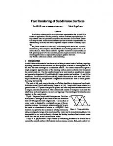
Figure 1: Bounded curvature Catmull-Clark [Augsd¨orfer et al., 2006] applied to an elliptic shape with an extraordinary vertex of valency eight at its centre. In each case the rendered surface is shown on left, and the polygon edges in the centre and at right. (a) basic subdivision, (b) vertices pushed to the limit surface, (c) adaptive subdivision, (d) B´ezier curves on spoke edges, (e) B´ezier patches between spoke edges.
6 in the same way. These facts make it relatively easy to implement adaptive subdivision to solve the rendering artifact problem compared with implementing general adaptive subdivision. As an example, assume that all edges in the base mesh are of roughly the same length and that n subdivision steps are sufficient in the regular regions of the mesh. The spoke edges (those emanating from the extraordinary vertex) will be too long. Assume that n is sufficiently large that the polygons in the 2-ring are sufficiently small. The ratio of edge lengths between polygons in the 2-ring and polygons in the 1-ring is approximately γ = (1 − λ )/λ . Adaptive subdivision thus needs to ensure that the maximum edge length is γ times the spoke edge length. For λ = 0.9, γ = 1/9. Figure 1(c) shows an example. This produces a rendered solution which is a visually acceptable approximation to the limit surface and thus solves the polar artifact problem. It has the practical drawback that some of the polygons near the extraordinary vertex are extremely small. Stam’s exact evaluation [Stam, 1998] is another method that is obviously relevant. If we polygonize the region around the extraordinary vertex in a uniform fashion, as illustrated in Figure 1(e), then we can evaluate the limit surface at every vertex of that polygonization. The issues here are that we need to handle Stam’s evaluation to high depths for high λ (at least 21 steps for the λ = 0.9 example above), that we need to precalculate and store all of the necessary matrices, and that we should ideally store a uniform mesh for each valency of extraordinary vertex. This is time-consuming to implement. The uniform polygonization in the parameter space can be generated easily enough by placing vertices at steps of γ along each spoke edge, joining these by transverse edges divided into steps no longer than γ and then connecting vertices on adjacent transverse edges in an appropriate way (Figure 1(e)). For a sufficiently fine polygonization, this clearly produces a surface which is indistinguishable from the limit surface and indistinguishable from the surface in Figure 1(c). It improves on adaptive subdivision by not generating a large number of tiny polygons. However, we would prefer a solution which is easier to implement and faster to evaluate than either of these methods. Exact evaluation of an approximate curved surface produces an adequate approximation to the limit surface without generating tiny polygons and without the need to perform Stam’s exact evaluation. We approximate the limit surface around the extraordinary vertex by Hermite interpolation, using a set of B´ezier triangles, and we sample off this approximation. Provided that the B´ezier triangles give a sufficiently good approximation to the limit surface, this will provide sufficiently good results. An early idea was to approximate the spoke edges by quadratic B´ezier curves. The end points were the vertices pushed onto the limit surface. The third control point could be determined in several ways. It is possible to find the tangent planes at the two end points, using the two eigenvectors corresponding to the two subdominant eigenvalues, λ . We defined the third control point to be the point on the intersection line of the two tangent planes that lies closest to the straight line joining the end points. Using these quadratic B´ezier curves, we could determine points at appropriate intervals along the curve, as shown in Figure 1(d). However, for all but very high valency, the triangles created between the spokes were too large, causing rendering artifacts. We propose, therefore, to use B´ezier triangles. The three corners of the triangle are the extraordinary vertex and two adjacent vertices in the 2-ring, all pushed onto the limit surface. We use vertices in the 2-ring so that the B´ezier triangles cover the entirety of the quadrilaterals surrounding the extraordinary vertex. The three other control points of the quadratic B´ezier triangles are determined analogously to the B´ezier curves, above. We use the same uniform polygonization as in Stam’s exact evaluation, at lower computational cost, with
7 the result shown in Figure 1(e). This only has a guarantee of C0 continuity across the spoke edges, but the angles between the tangent planes of adjacent B´ezier triangles is significantly less than between the facets that are actually being rendered.
3 Conclusion High values of λ are required to get limit surfaces with optimal properties around extraordinary vertices. The polar rendering artifacts which occur around extraordinary vertices for high λ can be removed by providing a better approximation to the limit surface than is given by subdividing a small number of times. Adaptive subdivision, Stam’s exact evaluation, and B´ezier triangle evaluation all provide a good approximation to the limit surface and visual smoothness. Any of these solutions allows subdivision schemes to use high values of λ without introducing polar artifacts into the rendered approximation of the limit surface, thus allowing us to achieve highest quality by using optimal values for λ .
References Ursula H. Augsd¨orfer, Neil A. Dodgson, and Malcolm A. Sabin. Tuning subdivision by minimising gaussian curvature variation near extraordinary vertices. Computer Graphics Forum, 25(3):263–272, 2006. Lo¨ıc Barthe and Leif Kobbelt. Subdivision scheme tuning around extraordinary vertices. Comp. Aided Geom. Des., 21:561 – 583, 2004. H. M¨uller and R. Jaeschke. Adaptive subdivision curves and surfaces. Technical Report No. 676, Universit¨at Dortmund, 1998. T. Ni and A. H. Nasri. Tuned ternary quad subdivision. In Geometric Modelling and Processing, volume 4077 of L. Notes in Comp. Sci., pages 441–450. Springer, 2006. ISBN 978-3-54036711-6. Malcolm Sabin and Lo¨ıc Barthe. Artifacts in recursive subdivision surfaces. In Curve and Surface Fitting: Saint-Malo 2002, pages 353–362. Nashboro Press, 2003. Jos Stam. Exact evaluation of Catmull-Clark subdivision surfaces at arbitrary parameter values. In Proc. ACM SIGGRAPH 98, pages 395–404. ACM Press, 1998. D. Zorin and P. Schr¨oder. Subdivision for modelling and animation. In SIGGRAPH 2000 Course Notes. ACM Press, 2000. Avi Zulti, Adi Levin, David Levin, and Mina Teicher. C2 subdivision over triangulations with one extraordinary point. Comp. Aided Geom. Des., 23:157–178, 2006.