Finite-Difference Methods,â SIAM Journal on Scientific Computing, Vol. 22, No. 5, 2001, pp. 1675â1696. 3Kreiss, H.-O. and Scherer, G., Finite Element and Finite ...
AIAA 2009-3658
19th AIAA Computational Fluid Dynamics 22 - 25 June 2009, San Antonio, Texas
Interface and Boundary Schemes for High-Order Methods Xun Huan,∗ Jason E. Hicken,† and David W. Zingg‡ Institute for Aerospace Studies, University of Toronto 4925 Dufferin St., Toronto, Ontario, Canada, M3H 5T6
High-order finite-difference methods show promise for delivering efficiency improvements in some applications of computational fluid dynamics. Their accuracy and efficiency are dependent on the treatment of boundaries and interfaces. Interface schemes that do not involve halo nodes offer several advantages. In particular, they are an effective means of dealing with mesh nonsmoothness, which can arise from the geometry definition or mesh topology. In this paper, two such interface schemes are compared for a hyperbolic problem. Both schemes are stable and provide the required order of accuracy to preserve the desired global order. The first uses standard difference operators up to third-order global accuracy and special near-boundary operators to preserve stability for fifth-order global accuracy. The second scheme combines summation-by-parts operators with simultaneous approximation terms at interfaces and boundaries. The results demonstrate the effectiveness of both approaches in achieving their prescribed orders of accuracy and quantify the error associated with the introduction of interfaces. Overall, these schemes offer several advantages, and the error introduced at mesh interfaces is small. Hence they provide a highly competitive option for dealing with mesh interfaces and boundary conditions in high-order multiblock solvers, with the summation-by-parts approach with simultaneous approximation terms preferred for its more rigorous stability properties.
I.
Introduction
In computational fluid dynamics there remains a need for more efficient algorithms driven by, for example, the following considerations: • The results of the recent drag prediction workshops indicating that with current solvers extremely fine meshes are required to achieve mesh-independent solutions. • The emergence of aerodynamic shape optimization and multidisciplinary optimization, which necessitate repeated flow solutions. • The need to go beyond the Reynolds-averaged Navier-Stokes (RANS) equations toward large-eddy and direct simulations of turbulent flows in some applications, such as combustion and aeroacoustics. One avenue by which algorithmic efficiency can be improved is through high-order methods. Initially, these were typically applied to unsteady problems requiring high accuracy. Subsequently, De Rango and Zingg1 demonstrated that high-order methods can be advantageous even in the solution of the steady RANS equations. Currently, development of efficient high-order finite-volume and finite-element methods is an active area of research. However, finite-difference methods also merit consideration, given their innate efficiency, i.e. high accuracy per unit cost. Their primary shortcoming is their restriction to structured meshes, but the advantages of unstructured meshes in terms of ease of generation have not materialized to the extent expected, so this limitation need not disqualify them from consideration. ∗ Undergraduate
Student (currently a Graduate Student at MIT), Student Member AIAA. Student, Student Member AIAA. ‡ Professor and Director, Canada Research Chair in Computational Aerodynamics, Associate Fellow AIAA. † Graduate
1 of 10 American of Aeronautics and Inc., Astronautics Copyright © 2009 by David W. Zingg. Published by the American InstituteInstitute of Aeronautics and Astronautics, with permission.
High-order finite-difference methods require boundary and interface schemes that preserve the desired global order of accuracy and maintain stability. Interface schemes are needed because most geometries of interest require the use of multi-block grids, typically either overlapping or patched - we will focus on the latter here. An obvious choice for interfaces is to utilize halo nodes such that the interior operator can be used at interfaces, and the interface is thus transparent. However, this approach has some shortcomings. First, special interface points (e.g. points with five neighbours) can exist where the interior operator cannot be used. Moreover, it can be difficult to ensure mesh smoothness across interfaces, and significant errors can occur if the mesh is not smooth. Furthermore, the halo node approach requires quite a bit of information to be passed between blocks, which can be detrimental to parallel performance, and the amount of information to be passed depends on the order of the operator. Consequently, we consider interface schemes that do not require halo nodes. Besides addressing the disadvantages listed above, this approach provides additional flexibility in the meshes on either side of the interface, which do not even require point continuity. Another prospective advantage arises in handling geometries that have either inherent discontinuities (e.g. in slope) or have limited differentiability arising from the geometry definition (e.g. NURBS or any piecewise function). By placing an interface at the discontinuity, the problem of differentiating across a discontinuity is removed. We consider two approaches to interface schemes without halo nodes. The first is due to Jurgens and Zingg,2 who applied high-order methods to the numerical solution of the time-domain Maxwell equations governing electromagnetic waves. In this application, one cannot differentiate across material interfaces, and the interface scheme must be properly designed to account for this. The interface approach of Jurgens and Zingg is designed to be used in conjunction with standard interior differencing schemes. An alternative approach is to combine summation-by-parts (SBP) operators with simultaneous approximation terms (SATs). SBP operators are derived from the energy method, first by Kreiss and Scherer3, 4 for low orders, and then by Strand5 for higher orders. SBP operators allow an energy estimate of the discrete form, potentially guaranteeing strict stability. However, boundary operators are needed, and these can destroy the SBP property.6–8 With the aim of preserving the SBP property of the overall scheme, the projection method9, 10 and the SAT approach6 have been developed. The projection method, while strictly stable for hyperbolic PDEs, becomes unstable for the linear convection-diffusion equation.7 A modified projection method, which is a hybrid between the injection and projection methods, destroys the SBP property but still offers strict stability.7, 11 The SAT method, based on a boundary value penalty method, does not have these stability problems, and has been studied extensively.12, 13 A systematic comparison between the injection, projection, modified-projection, and SAT methods has been made by Strand.14 SAT interfaces have previously been studied in the context of the one-dimensional constant-coefficient Euler and NavierStokes equations,15 the Burgers equation,16 linear scalar problems in multi-dimensions and curvilinear coordinates,17 the three-dimensional Euler equations with parallelization,18 and the compressible Navier-Stokes equations.19 For nonlinear systems, artificial dissipation is needed to improve stability, especially when centereddifference schemes and explicit time-marching methods are used. Scalar and matrix dissipation models have been studied,20–23 and various boundary modifications have been proposed to increase compatibility with the SBP operators.24 Dissipation schemes preserving the SBP property have been studied by Olsson25 and Strand.14 Mattsson et al.26 developed stable dissipation operators specifically for SBP schemes with the SAT treatment, accurate to any arbitrary order. In the present work, only the traditional matrix dissipation model is implemented. The objective of this paper is to compare the accuracy of difference operators using the boundary and interface schemes of Jurgens and Zingg2 (referred to as “conventional schemes”) with SBP schemes using the SAT approach to boundaries and interfaces (referred to as “SBP schemes”). The comparison is performed in the context of the quasi-one-dimensional Euler equations.
II.
Quasi-One-Dimensional Euler Equations
The quasi-one-dimensional Euler equations governing (approximately) the flow in a converging-diverging nozzle are given by ∂Q ∂f + =g ∂t ∂x
2 of 10 American Institute of Aeronautics and Astronautics
(1)
where Q is the vector of conservative variables, f defined as ρS Q = ρuS ρES
is the flux-vector, and g is the source term. They are q1 = q2 q3
(2)
q2 ρuS (γ−3) q22 2 (γ − 1)q f = (ρu + p)S = 3− 2 q1 3 γ−1 q2 γq3 q2 ρuHS − q1 2 q2
1
0
g = p dS dx 0
0 1 dS = S dx (γ − 1)(q3 −
2 1 q2 2 q1 )
0
(3)
(4)
where H = E + p/ρ. The system is closed by assuming a perfect gas. The function S(x) is the cross-sectional area of the nozzle. Two different definitions for S(x) are explored here, each with a different degree of continuity in the derivative of the function. Shape 1 is a C ∞ continuous area, defined by: S(x) =
−1 3 1 7 5 x + x2 − x + 250 10 10 2
Shape 2 is a C 2 continuous area, defined by: ' 7 2 1 x3 + 50 x − 54 x + − 125 S(x) = 1 2 1 3 50 x − 5 x + 2
5 2
for 0 ≤ x ≤ 10
for 0 ≤ x ≤ 5 for 5 < x ≤ 10
(5)
(6)
The third derivative is discontinuous at x = 5. Many piecewise geometry representations are C 2 continuous, as exemplified by this function. The nozzle flow is uniquely determined by the following boundary conditions, which correspond to a subsonic flow:
III. A.
pin Tin
= 100, 000 Pa = 200 K
pout
= 92, 772 Pa
Numerical Methods
Conventional Schemes
We consider centered interior schemes of second, fourth, and sixth order. The second-order scheme is combined with third-order matrix artificial dissipation, giving a scheme with second-order global accuracy, as long as the boundary and interface schemes are at least first-order accurate. The fourth-order scheme is combined with the same third-order dissipation. Hence this scheme is third-order globally and requires boundary and interface schemes of at least second-order. The sixth-order operator is combined with fifthorder dissipation; when combined with boundary and interface operators of at least fourth-order, this leads to fifth-order global accuracy. Boundary and interface conditions are implemented using Riemann invariants. For example, at an interface, two Riemann invariants are extrapolated to the interface from the upstream block (using an extrapolation method of appropriate order of accuracy), and one is extrapolated from the downstream block. This is sufficient to define the state at the interface.
3 of 10 American Institute of Aeronautics and Astronautics
(a) Subdomains for conventional schemes
(b) Subdomains for SBP schemes
Figure 1. Example domain consisting of two equal-size and equal-resolution subdomains with an interface
The fourth-order centered interior operator is stable in combination with the following biased scheme at the first interior node to the right of a boundary or an interface: ( ) −1 1 1 1 (7) f0 − f1 + f2 − f3 (δx f )1 = ∆x 3 2 6 with the equivalent operator used at the interior node to the left of a boundary or interface (see Fig. 1(a)). For the globally fifth-order scheme, different boundary and interface operators are used, depending on the wave direction. This is implemented using flux-vector splitting. At the first two interior nodes, standard fifth-order upwind-biased formulas are used for the outgoing waves: ( ) + * 1 −1 − 13 − 1 1 δx f − 1 = (8) f0 − f1 + 2f2− − f3− + f4− − f5− ∆x 5 12 3 20 ( ) + * 1 − 1 − 1 − 1 1 1 (9) f0 − f1 − f2 + f3− − f4− + f5− δx f − 2 = ∆x 20 2 3 4 30 For incoming waves, the following formulas are used in order to provide stability in conjunction with sixthorder centered differences in the interior:2 ( ) + * 1 −1 + 119 + 17 + 57 3 31 (10) δx f + 1 = f0 − f1 + f2 − 4f3+ + f4+ − f5+ + f6+ ∆x 20 60 4 12 60 20 ) ( + * 1 3 + 11 + 7 + 5 17 1 δx f + 2 = (11) f0 − f1 + f2 − f3+ + f4+ − f5+ + f6+ ∆x 20 10 6 4 30 10
Analogous formulas are used at the two nodes to the left of a boundary or interface. B. 1.
SBP Schemes Single Domain
* + The SBP operator approximates the first derivative of a scalar quantity ux through P −1 Q u; the P matrix is also called the norm matrix. Since the Euler equations are a system of equations, the operator needs to be modified through a tensor product. For the remainder of the paper, P refers to (P ⊗ I) and Q to (Q ⊗ I), where I is a 3 × 3 identity matrix. Various norms are available to satisfy the SBP property. In particular, the restricted-full norm is advantageous over the full norm because the former can be shown to be stable for first-order hyperbolic systems, but the latter cannot.5 However, both of these two norms lose stability for curvilinear grids, while the diagonal norm recovers stability.28 The disadvantage of the diagonal norm is that the interior scheme needs to be twice the order of the boundary scheme; this becomes increasingly disadvantageous as the order is increased. In this work, the diagonal norm is implemented for its simplicity as well as its potential advantages on curvilinear grids. When the SBP scheme is applied, the SAT boundary treatment is used in order to preserve the SBP property of the overall scheme. The SAT formulation modifies the semi-discrete form of the PDE with penalty terms proportional to the difference between the computed values of the boundary nodes and the
4 of 10 American Institute of Aeronautics and Astronautics
boundary conditions. This is applied after the original semi-discrete form is premultiplied by the P matrix, giving dQ = −Qf + Pg + W(Q − Qbc ) (12) P dt The boundary condition vector Qbc is defined as (Qbc )1 0 . .. Qbc = (13) 0 (Qbc )N
where (Qbc )1 and (Qbc )N are the boundary conditions on the left and right boundaries, respectively. The weight matrix W is defined as wL 0 .. (14) W= . 0 wR
where wL and wR are the 3 × 3 matrix weights of the penalties applied at the left and right boundaries, respectively. For the Euler equations, we have chosen18 wL wR
1, |A| 12 + A 21 2 1, |A|N + 12 − AN + 21 = − 2
= −
(15) (16)
where |A| and A are calculated at an averaged state between the boundary state and the target boundary state, which differ slightly as a result of the use of SATs . The entries for the P and P −1 Q matrices can be found in the Appendix of works by Olsson29 and Strand.5 The minimal bandwidth 4th-order schemes and the minimal spectral radius 5th-order schemes are used.30 Third-order matrix dissipation is added to the second- and third-order SBP schemes, and fifth-order dissipation is added to the fourth- and fifth-order schemes. 2.
Multiple Subdomains
An example of a two-subdomain case using SBP operators is shown in Fig. 1(b). Two sets of values, at nodes i and i + 1, are needed to represent the interface node. We shall adopt a treatment that is analogous to the boundary treatment. For example, in constructing two subdomains, we have the following derivation dQL dt dQR PR dt PL
=
−QL fL + PL gL + WL (QL − Qbc,L )
(17)
=
−QR fR + PR gR + WR (QR − Qbc,R )
(18)
where WL and WR are analogous to W in Eq. 12, Qbc,L contains the left-hand boundary values in its first entry and Qi+1 in its last entry, and Qbc,R contains Qi in its first entry and the right-hand boundary values in its last entry. Equations 17 and 18 can be combined into a form similar to Eq. 12. The main modification
5 of 10 American Institute of Aeronautics and Astronautics
Scheme
Conventional
SBP
2nd-order 3rd-order 4th-order 5th-order
B=1, I=2, D=3 B=2, I=4, D=3 – B=5, I=6, D=5
B=1, B=2, B=3, B=4,
I=2, I=4, I=6, I=8,
D=3 D=3 D=5 D=5
Table 1. Boundary (B), interior (I), and dissipation (D) scheme orders
occurs to the weight matrix: wL W=
0 ..
. 0 w1 −w2
−w1 w2 0 ..
. 0 wR
The interface weights are analogous to the boundary weights: w1 w2
1, |A|i+ 12 − Ai+ 12 2 1, = − |A|i+ 12 + Ai+ 12 2
= −
1 2 .. . i−1 i i+1 i+2 .. .
(19)
N N +1
(20) (21)
In effect, Qi+1 provides the right-hand boundary condition for the left subdomain, and Qi provides the lefthand boundary condition for the right subdomain. Schemes with more subdomains are developed similarly.
IV.
Results
We investigate the accuracy of the conventional and SBP schemes applied to the quasi-one-dimensional Euler equations by examining the root-mean-square errors in pressure on a sequence of meshes with varying densities for the two nozzle cross-sectional area definitions described by Eqns. 5 and 6. Table 1 summarizes the theoretical orders of accuracy of the interior and boundary schemes compared. As a result of the choice of the diagonal norm, the SBP schemes have an interior scheme that has an order of accuracy twice that of the boundary scheme. This is higher than needed to achieve the desired global order of accuracy but required for stability on curvilinear grids. Consequently, the stability bound for the fifth-order SBP scheme is a bit lower than that for the fifth-order conventional scheme if explicit time-marching is used. The conventional scheme has no guarantee of stability on curvilinear grids, but has been successfully used on such grids by Jurgens and Zingg.2 The increased stencil size in the interior associated with the fifth-order SBP scheme is a potential disadvantage with respect to speed and memory (increased matrix bandwidth for implicit methods), but this is balanced by its more rigorous stability properties. A.
Single Domain
The error plots for a single domain (i.e. a domain with no interfaces) are presented in Fig. 2, and the observed orders of accuracy are summarized in Table 2. For shape 1, all schemes yield their expected accuracy orders. Comparing the conventional and SBP scheme error plots, the accuracy of these schemes is very close except for the 5th-order scheme, where the
6 of 10 American Institute of Aeronautics and Astronautics
−2
10
10
−4
10
RMS Error of Pressure
RMS Error of Pressure
10
−6
10
−8
10
−10
10
2nd−Order Conv. 3rd−Order Conv. 5th−Order Conv. 2nd−Order SBP 3rd−Order SBP 4th−Order SBP 5th−Order SBP
−12
10
−14
10
−16
10
10
1
10 10 10 10 10 10
2
3
10 Number of Nodes
−2 −4 −6 −8 −10
2nd−Order Conv. 3rd−Order Conv. 5th−Order Conv. 2nd−Order SBP 3rd−Order SBP 4th−Order SBP 5th−Order SBP
−12 −14 −16 1
10
2
10
3
10 Number of Nodes
(a) Shape 1
10
(b) Shape 2
Figure 2. Errors for a single domain - shapes 1 (C ∞ ) and 2 (C 2 )
Conventional
SBP
Shape
2nd-Order
3rd-Order
5th-Order
2nd-Order
3rd-Order
4th-Order
5th-Order
1 2
2.03 2.03
3.16 3.19
5.35 3.75
2.02 2.03
3.24 3.34
4.53 3.68
5.10 3.55
Table 2. Orders of accuracy for a single domain - shapes 1 and 2
SBP scheme is slightly more accurate than its conventional counterpart, presumably due to its higher order in the interior. For shape 2, the 2nd- and 3rd-order schemes have the prescribed accuracy orders, but the 4th- and 5th-order schemes display a reduced order of accuracy due to the discontinuity in the third derivative of the nozzle area function. B.
Multiple Subdomains
In this section, we investigate the accuracy of the interface schemes by introducing multiple subdomains. Initially, the number of subdomains is fixed, while the number of nodes per subdomain is varied. The analysis is performed with 2, 3, 4, 5, 8, and 16 subdomains for shapes 1 and 2. The orders of accuracy are summarized in Tables 3 and 4. In a second study, the total number of nodes is held fixed at 721, while the number of subdomains is varied; these results are presented in Fig. 3. Table 3 shows that for shape 1 the design orders of accuracy are achieved or exceeded. For shape 2 there is a reduction in order in the 4th- and 5th-order schemes when the number of subdomains is odd, as with a single domain, but the design order is recovered when the number of subdomains is even. In the latter case, an interface is located at x = 5, where the discontinuity in the third derivative of the area function occurs. Fig. 3(a) shows the effect of introducing interfaces on each method for the C ∞ continuous nozzle. The error increases modestly with the number of interfaces. This occurs as a result of the fact that the interface schemes are generally less accurate than the interior schemes. The conventional and SBP schemes perform similarly in this regard, although the conventional third-order scheme has a higher error with multiple subdomains than its SBP counterpart. Overall, the increase in error with an increasing number of subdomains is modest and consistent with the global order of the scheme. Fig. 3(b) again shows that the fourth-order and especially the fifth-order schemes are significantly more accurate when the number of subdomains is even and there is thus an interface at the discontinuity. The ability to achieve 4th- and 5th-order accuracy for a C 2 continuous geometry (or even a C 1 continuous geometry or mesh) is an important advantage of both of these schemes compared to schemes based on halo nodes.
7 of 10 American Institute of Aeronautics and Astronautics
Conventional
SBP
# Subdomains
2nd-Order
3rd-Order
5th-Order
2nd-Order
3rd-Order
4th-Order
5th-Order
2 3 4 5 8 16
2.03 2.02 2.02 2.02 2.02 2.03
3.24 2.96 3.08 2.94 2.95 2.89
5.11 5.16 5.15 5.01 5.11 5.00
2.03 2.04 2.03 2.03 2.04 2.04
3.32 3.36 3.33 3.33 3.29 3.22
4.56 4.78 4.55 4.56 4.48 4.44
5.12 5.25 5.08 5.24 5.18 5.10
Table 3. Orders of accuracy for 2, 3, 4, 5, 8, and 16 subdomains - shape 1
Conventional
SBP
# Subdomains
2nd-Order
3rd-Order
5th-Order
2nd-Order
3rd-Order
4th-Order
5th-Order
2 3 4 5 8 16
2.03 2.02 2.02 2.02 2.02 2.03
3.00 2.91 2.96 2.95 2.88 2.85
5.17 3.79 5.16 3.99 4.89 4.92
2.03 2.03 2.03 2.03 2.03 2.03
3.42 3.43 3.42 3.40 3.36 3.28
4.66 4.24 4.63 4.21 4.47 4.44
5.18 3.58 5.22 3.52 5.17 5.16
Table 4. Orders of accuracy for 2, 3, 4, 5, 8, and 16 subdomains - shape 2
2nd−Order Conv. 3rd−Order Conv. 5th−Order Conv. 2nd−Order SBP 3rd−Order SBP 4th−Order SBP 5th−Order SBP
RMS Error
−5
2nd−Order Conv. 3rd−Order Conv. 5th−Order Conv. 2nd−Order SBP 3rd−Order SBP 4th−Order SBP 5th−Order SBP
0
10
RMS Error
0
10
10
−10
10
−5
10
−10
10 0
5 10 Number of Subdomains
15
0
(a) Shape 1
5 10 Number of Subdomains
15
(b) Shape 2
Figure 3. Errors as a function of number of subdomains - shapes 1 and 2
V.
Conclusions
We have compared two boundary and interface schemes, a conventional scheme and an SBP scheme with SATs, which do not require halo nodes at block interfaces. These approaches have several advantages. They are particularly useful if the geometry or mesh has some sort of discontinuity. Higher-order finite-difference methods require a higher degree of continuity than their lower-order counterparts, and if the required degree of continuity is not present, then a reduction in order will be seen. With the interface schemes studied here, this reduction in order can be avoided by introducing an interface at the location of the discontinuity. Moreover, these schemes do not require mesh continuity across block interfaces, which can be difficult to
8 of 10 American Institute of Aeronautics and Astronautics
achieve, and involve reduced interblock communication for parallel solvers. The results demonstrate the effectiveness of both approaches in achieving their prescribed orders of accuracy and quantify the error associated with the introduction of interfaces. The SBP-SAT approach is somewhat more accurate and has more rigorous stability properties. For the two fifth-order schemes specifically, the conventional scheme has a smaller interior stencil size and a slightly increased stability bound when explicit time-marching is used. Overall, these schemes offer several advantages, and the additional error introduced is small. Hence they provide an appealing option for dealing with block interfaces in multiblock solvers. In particular, the SBP-SAT approach is preferred because it can be readily extended to arbitrary orders of accuracy.
Acknowledgments The authors acknowledge financial assistance from the Natural Science and Engineering Research Council (NSERC), the Canada Research Chairs program, and the University of Toronto.
References 1 De
Rango, S., and Zingg, D.W., “A High-Order Spatial Discretization for Turbulent Aerodynamic Computations”, AIAA J., Vol. 39, No. 7, 2001, pp. 1296-1304. 2 Jurgens, H. M. and Zingg, D. W., “Numerical Solution of the Time-Domain Maxwell Equations Using High-Accuracy Finite-Difference Methods,” SIAM Journal on Scientific Computing, Vol. 22, No. 5, 2001, pp. 1675–1696. 3 Kreiss, H.-O. and Scherer, G., Finite Element and Finite Difference Methods for Hyperbolic Partial Differential Equations, Mathematical Aspects of Finite Elements in Partial Differential Equations, Academic Press, New York, 1974. 4 Kreiss, H.-O. and Scherer, G., “On the Existence of Energy Estimates for Difference Approximations for Hyperbolic Systems,” Tech. Rep. Dept. of Scientific Computing, Uppsala University, 1977. 5 Strand, B., “Summation by Parts for Finite Difference Approximations for d/dx,” J. Comput. Phys., Vol. 110, No. 1, 1994, pp. 47–67. 6 Carpenter, M. H., Gottlieb, D., and Abarbanel, S., “Time-Stable Boundary Conditions for Finite-Difference Schemes Solving Hyperbolic Systems,” Journal of Computational Physics, Vol. 111, No. 2, 1994, pp. 220–236. 7 Mattsson, K., “Boundary Procedures for Summation-by-Parts Operators,” SIAM Journal on Scientific Computing, Vol. 18, No. 1, 2003, pp. 133–153. 8 Gustafsson, B., Kreiss, H.-O., and Oliger, J., Time Dependent Problems and Difference Methods, Wiley, 1995. 9 Olsson, P., “Summation by Parts, Projections, and Stability. I,” Mathematics of Computation, Vol. 64, No. 211, 1995, pp. 1035–1065. 10 Olsson, P., “Summation by Parts, Projections, and Stability. II,” Mathematics of Computation, Vol. 64, No. 212, 1995, pp. 1473–1493. 11 Gustafsson, B., “On the Implementation of Boundary Conditions for the Method of Lines,” Tech. Rep. 195, Dept. of Scientific Computing, Uppsala University, 1997. 12 Abarbanel, S. and Ditkowski, A., “Asymptotically Stable Fourth-Order Accurate Schemes for the Diffusion Equation on Complex Shapes,” Journal of Computational Physics, Vol. 133, No. 2, 1997, pp. 279–288. 13 Johansson, S., “Numerical Solution of the Linearized Euler Equations Using High Order Finite Difference Operators with the Summation by Parts Property,” Tech. Rep. Report No. 2002-034, Dept. of Information Technology, Uppsala University, October 2002. 14 Strand, B., High-Order Difference Approximations for Hyperbolic Initial Boundary Value Problems, Ph.D. thesis, Uppsala University, 1996. 15 Nordstr¨ om, J. and Carpenter, M. H., “Boundary and Interface Conditions for High-Order Finite-Difference Methods Applied to the Euler and Navier-Stokes Equations,” Journal of Computational Physics, Vol. 148, No. 2, 1999, pp. 621–645. 16 Carpenter, M. H., Nordstrom, J., and Gottlieb, D., “A Stable and Conservative Interface Treatment of Arbitrary Spatial Accuracy,” SIAM Journal on Scientific Computing, Vol. 148, 1999, pp. 341–365. 17 Nordstr¨ om, J. and Carpenter, M. H., “High-Order Finite Difference Methods, Multidimensional Linear Problems, and Curvilinear Coordinates,” Journal of Computational Physics, Vol. 173, No. 1, 2001, pp. 149–174. 18 Hicken, J. E. and Zingg, D. W., “A Parallel Newton-Krylov solver for the Euler Equations Discretized Using Simultaneous Approximation Terms,” AIAA J., Vol. 46, No. 11, 2008, pp. 2773-2786. 19 Svard, M., Carpenter, M.H., and Nordstrom, J., “A Stable High-Order Finite Difference Scheme for the compressible Navier-Stokes Equations, far-field boundary conditions,” Journal of Computational Physics, Vol. 225, No. 1, 2007, pp. 1020– 1038. 20 Swanson, R. C. and Turkel, E., “On Central-Difference and Upwind Schemes,” Journal of Computational Physics, Vol. 101, 1992, pp. 292–306. 21 Swanson, R. C., Radespiel, R., and Turkel, E., “Comparison of Several Dissipation Algorithms for Central Difference Schemes,” Report 97-40, ICASE, August 1997. 22 Zingg, D. W., Lomax, H., and Jurgens, H., “High-Accuracy Finite-Difference Schemes for Linear Wave Propagation,” SIAM Journal on Scientific Computing, Vol. 17, No. 2, 1996, pp. 328–346. 23 Zingg, D. W., De Rango, S., Nemec, M., and Pulliam, T. H., “Comparison of Several Spatial Discretizations for the Navier-Stokes Equations,” Journal of Computational Physics, Vol. 160, 2000, pp. 683–704.
9 of 10 American Institute of Aeronautics and Astronautics
24 Olsson, P. and Johnson, S. L., “Boundary Modifications of the Dissipation Operators for the Three-Dimensional Euler Equations,” SIAM Journal on Scientific Computing, Vol. 4, No. 2, 1989, pp. 159–195. 25 Olsson, P., High-Order Difference Methods and Dataparallel Implementation, Ph.D. thesis, Uppsala University, 1992. 26 Mattsson, K., Sv¨ ard, M., and Nordstr¨ om, J., “Stable and Accurate Artificial Dissipation,” SIAM Journal on Scientific Computing, Vol. 21, No. 1, 2004, pp. 57–79. 27 Gustafsson, B., “The Convergence Rate for Difference Approximations to Mixed Initial Boundary Value Problems,” Mathematics of Computation, Vol. 29, No. 130, April 1975, pp. 396–406. 28 Sv¨ ard, M., “On Coordinate Transformations for Summation-by-Parts Operators,” SIAM Journal on Scientific Computing, Vol. 20, No. 1, 2004, pp. 29–42. 29 Olsson, P., “Stable Approximation of Symmetric Hyperbolic and Parabolic Equations in Several Space Dimensions,” Tech. Rep. Report No. 138, Dept. of Scientific Computing, Uppsala University, February 1992. 30 Sv¨ ard, M., Mattsson, K., and Nordstr¨ om, J., “Steady-State Computations Using Summation-by-Parts Operators,” SIAM Journal on Scientific Computing, Vol. 24, No. 1, 2005, pp. 647–663.
10 of 10 American Institute of Aeronautics and Astronautics