The rainfall-runoff model is TopModel (Beven, 1997) and the ... Once the systems' interacting physical quantities and coupling surfaces have been identified, the next step is to ..... Modelling and Software Society, iEMSs: Osnabrück, Germany.
Interface-based Support for Model Coupling: Spatial Representation and Compatibility Issues Tom Bulatewicz and Janice Cuny Department of Computer and Information Sciences, University of Oregon, Eugene, OR 97403 Tel: +1 541-346-4408 FAX: +1 541-346-5373 Email: {tomb, cuny}@cs.uoregon.edu
Abstract Model coupling is a nontrivial task that is not adequately supported in existing frameworks. Our long-term goal is to support the fast-prototyping of model couplings, enabling scientists to quickly experiment with a variety of linkings without having to make an upfront investment in reprogramming. The centerpiece of our framework, the Potential Coupling Interface (PCI), must expose all the characteristics of a model that are relevant to model coupling, but what are those characteristics? To explore different couplings, and to identify the relevant model characteristics, we conducted a study of 14 hydrological models and the pairwise couplings between them. We found that the model characteristics relevant to coupling lie in four dimensions: space, time, structure, and data. Models of the same phenomena often had similar characteristics, making it feasible to replace them within a coupling when appropriate for specific sites. We also found that resolving differences along the four dimensions, particularly with respect to space, can be complex.
1. Introduction Modeling and simulation are important tools of research in nearly every physical science. In many domains - and certainly in our target domain of Hydrology - validated models of a variety of phenomena already exist, and the current challenge is to integrate or couple them into models of more complex, interacting physical systems. The straightforward approach of merging a set of model codes into a single, monolithic program is time consuming and it requires a detailed knowledge of the individual codes. Once such an integrated program is created, it freezes the constituent codes, making it difficult to take advantage of any ongoing improvements to the original models, and making it difficult to replace one of the codes with an alternative that may be more appropriate for a particular site (Rowan, 2001). Our work, as well as work of others (MpCCI, 2005; Valcke et al., 2000; Blind and Gregersen, 2004; Armstrong et al., 2005; Leavesley et al., 1996), aims to build an infrastructure that supports a more modular, flexible approach to model coupling, allowing scientists to easily create and explore a variety of couplings. At the centerpiece of our work is a novel interface that we are designing, called the Potential Coupling Interface (PCI) (Bulatewicz et al., 2004). The PCI is an annotated flow graph of a model code that serves three roles in our infrastructure: first
it is a new form of metadata describing the potential ways in which a model can be used in a coupling; second it is the vehicle for the specification of how a set of coupled models interact with each other; and third it is the basis for automatic code generation that is used to instrument the original model codes. Here we focus on its use as metadata. Currently the PCI describes the overall model code structure, the data that is available for exchange with other models, and the locations in the model code where that data is accessible. This information is necessary for coupling, but it is not sufficient. The PCI does not yet capture needed information about the semantics of the model data, nor does it adequately support the identification and resolution of differences in these semantics between models. In order to complete the design of the PCI, we have studied a number of coupled models and hypothetical couplings of models commonly used in hydrological simulation. We report here on our findings regarding the relevant model characteristics that affect compatibility, and hence probable ease of coupling, of the models. In Section 2, we introduce the PCI and our approach with a case study of the coupling of two wellknown models. In Section 3, we assess the compatibility of the set of models in pairwise couplings, and in Section 4, we look more closely at the possible mechanisms for resolving incompatibilities, particularly with respect to spatial characteristics.
2. Case Study In this section we describe the coupling of a rainfall-runoff model with an aquifer model. (Note while it is possible to couple sets of models at a time, our discussion is clearer if we think of coupling as occurring between just two models.) The rainfall-runoff model is TopModel (Beven, 1997) and the aquifer model, ModFlow (McDonald and Harbaugh, 1988). TopModel is a 2-dimensional model of a catchment that calculates the amount of water exiting the catchment outlet in response to rainfall. ModFlow is a 3-dimensional aquifer model that simulates the height of the water table below the surface. Both models are distributed, time-dependent, written in Fortran, and possess the traditional input-compute-output model code structures. Both models begin by reading their input parameters and then execute a time-stepped loop, writing their results after each step, shown in Figure 1. Note though, that the models have different control structures, most importantly, TopModel executes its entire time-stepped loop for each subcatchment, while ModFlow progresses through its time-stepped loop just once.
Figure 1. ModFlow PCI (left) and TopModel PCI (right). Figure 1 shows the PCI for these models. PCIs are meant to be created just once, by the original programmer (or someone familiar with the model), as model metadata; after which they can be reused for any couplings. They look much like the flowcharts commonly found in model documentation. Our PCIs are generated automatically from user-annotated model codes and then edited to improve readability and to incorporate additional high-level information. Node labels and colors (grayscale in this figure) in the graph, supplied by the programmer, indicate the function of the code represented by the node. The graph depicts the overall control flow of the program with respect to potential coupling points. Arrows indicate the flow of control, and the dark arrows indicate potential coupling points, that is, places where the values of state variables - the variables that represent the state of the physical quantities being modeled - can be exchanged with other models. State variables cannot be accessed at arbitrary locations as they may have intermediate or inconsistent values. The variables available at each coupling point (as shown in the pop up boxes in the figure) are specified by the creator of the PCI. In order to demonstrate how the PCI is used, as well as its current limitations, we step through the design of a coupling between TopModel and ModFlow.1 We divide the task of creating a coupled model into five steps and present each one, first generally and then with respect to the case study. The first step occurs on the domain level, where the scientist must identify an interaction between physical systems that s/he wishes to study. The interactions - how the physical quantities of each system influence each other - can be unidirectional
1
This coupling was designed in collaboration with Alphonce Guzha, Utah State University, as part of a Hydrological study.
or bidirectional and they can take place continuously, or only at discrete points in time. The physical quantities themselves are usually spatially distributed, and they influence each other across a common physical boundary. The first step of model coupling then is the identification of this boundary, which we call the coupling surface. At one extreme the coupling surface is an adjacency; at the other, it is a complete overlap, the entire physical space simulated in both models. For the cases in between, the coupling surface is an overlapping region between the two modeled physical spaces. Step 1. What interactions between the physical systems are to be studied and where do these interactions occur? Case study: The runoff from a catchment is heavily influenced by both the rainfall over the catchment, as well the ground water beneath the catchment. When simulating the runoff from a catchment, TopModel makes very simple assumptions about the behavior of the ground water beneath it. In this coupling, we replace TopModel's simple ground water height calculations with ModFlow's full simulation of the saturated zone. The physical quantities involved are the water table height of the aquifer, and the unsaturated zone-saturated zone flow (we refer to this generally as recharge). These quantities influence each along the lower boundary of the catchment's unsaturated zone (TopModel) which is adjacent to the upper boundary of the aquifer (ModFlow). Once the systems' interacting physical quantities and coupling surfaces have been identified, the next step is to determine the state variables involved from each model code. Step 2. Which state variables represent the physic al quantities involved in the interaction? Case study: The water table height of the aquifer is represented by ModFlow's hnew array. The recharge between the catchment and the aquifer is represented by TopModel's quz variable. Unlike most coupling frameworks in which the interfaces between model components strictly enforce a common syntax and semantics for exchanging data (e.g. Blind and Gregersen, 2004), the data stored in the state variables of our PCIs have model-specific syntax and semantics, including, for example, associated units or spatial distribution, which must be accounted for in any coupling. Step 3. What are the syntax and semantics of each state variable? Case study: This step reveals an incompatibility in that ModFlow's water table height variable, hnew, is spatially distributed over a regular grid, while TopModel's recharge variable, quz, is spatially distributed over a set of irregularly shaped subcatchments. In order for these quantities to interact, their variables must be mapped to the same space. Here, each ModFlow cell must be mapped to the TopModel subcatchment(s) located above it. Next, the locations within each model code where the variables should be accessed for communication with the other model must be identified. From the PCI, we know where it's permissible to access variables within the individual model codes but not how those access points line up between the codes. Different access points within a model code correspond to different points in simulation time, and data exchanges must happen at the same (or at least coordinated) points in simulation time.
Step 4. Where in the model codes should the data exchanges between state variables take place? There are several places within a model code where a state variable is usable, each representing the variable at a different point in simulation time. For example, accessing a state variable at the start of a time step loop represents the state of a physical quantity at time T, while accessing that variable at the end of a time step loop represents the state of the quantity at time T+1. In order for the coupled models' interactions to be meaningful, the data exchanged must represent the same point in simulation time, and thus by extension, the locations chosen must provide/use the data at the same frequency. This highlights the importance of the surrounding control structure (loops, conditionals, etc.) when choosing the location(s) to access a variable. Case study: It is clear from the two PCIs that simply accessing state data at the start of each time step would not work because TopModel's time loop is within a spatial loop. As a result, each TopModel time step is simulated multiple times (once for each subcatchment), while each ModFlow time step is simulated only once. Furthermore, because groundwater moves much more slowly than surfacewater, the length of a ModFlow time step is longer than the length of a TopModel time step. These structural differences represent another incompatibility between the models. One way to resolve them is to have TopModel simulate all the subcatchments for a small set of short time steps for each long time step of ModFlow. In such a situation, the hnew variable of ModFlow would be accessed at the start of each time step, and the quz variable of TopModel would be accessed after the subcatchment loop (see Figure 1). As shown in this example, the models often need some control that was not in their original code; in this case, TopModel will have to execute its subcatchment loop many times, once for each iteration of ModFlow’s time step loop. In our infrastructure, as in most coupling frameworks (Valcke et al., 2000; MpCCI, 2005), this added control will reside in an intermediary application, called a coupler. Once the locations have been chosen where the relevant state variables should be accessed, the final step is to specify precisely how the state variables affect each other. Often the values of the state variables must be transformed before they can be used to affect each other. These transformations are functions, specified by the scientist, that compute new values for variables based on the values of variables from both models. If the data is spatially distributed, as part of this function, it may be necessary to map the simulation spaces to each other (see Section 4). Step 5. What is the quantitative relationship between the variables of each model? Case study: In this coupling, the subcatchments of TopModel are larger than the cells of ModFlow, and so the water table height must be averaged across all the cells beneath a subcatchment before it can be used by TopModel. In the reverse direction, the recharge from each subcatchment calculated by TopModel must be converted to a water table height value and then distributed among the set of cells of ModFlow located below that subcatchment. In either direction, the water table height must be adjusted for units, and additional calculations are necessary to relate the water table height to recharge. This completes the initial design of the model. We expect to support the design process and the subsequent implementation with our infrastructure. This case study highlights the kinds of incompatibilities that can arise when coupling models. Differences in code structure, grid scales and shapes, in time step lengths, and in units all influence the design of a coupled model. Although our
initial design of the PCI describes the structure and state variables of a model, it does not describe the other aspects of a model that play a role in coupling. In particular, much of the effort of creating a coupling will be spent on resolving model incompatibilities and we must insure that all of the necessary information to accomplish the resolution is available within the PCI. In order to better understand the range of incompatibilities that must be covered, we undertook an examination of common hydrological models and the pairwise couplings between them.
3. Coupled Model Study The purpose of this investigation was to identify the common characteristics of models that affect coupling compatibility and to assess the degree of compatibility of model pairs based on those characteristics. We restricted the study to a set of popular models within our application domain of Hydrology. Methodology. We studied a set of 14 hydrological models and the design of pairwise couplings between them. The models, which varied in complexity, were representative of the different kinds of systems commonly modeled in Hydrology: aquifer (A), streamflow (S), runoff (R), receiving water (W), and soil (O) systems, as shown in Table 1. Table 1. Models used in the coupling study Model BioMOC Branch DAFlow FourPt GLEAMS ModFlow OTIS SHAW STAMMT-L SWAT SWMM TopModel UEB WASP
Description Groundwater flow and solute transport Streamflow Streamflow Streamflow Soil chemistry and runoff Groundwater flow Stream solute transport Soil chemistry and runoff Stream solute transport Rainfall-runoff and solute transport Storm runoff Rainfall-runoff Snow-melt Receiving water
Kind A S S S O A S O S R R R R W
Reference Essaid and Bekins, 1997 Schaffranek et al., 1981 Jobson, 1989 DeLong et al., 1997 Leonard et al., 1987 McDonald and Harbaugh, 1988 Runkel, 1998 Flerchinger, 2000 Haggerty and Reeves, 2000 Neitsch et al., 1999 Huber and Dickinson, 1988 Beven, 1997 Tarboton et al., 1995 Ambrose et al., 1993
For each pairing of these models, we created the appropriate PCIs and used them to design a coupled model following the five steps described above. Results: The results of each step are presented here, and for each step, the key characteristics identified appear in bold in the text, and are summarized in Table 2. Step 1. What interactions between the physical systems are to be studied and where do these interactions occur? The physical systems simulated by the models in our set influence each other in many ways, but since water (represented as a height, flow rate, etc.) is the physical quantity
common to all the systems, we focused on water flux between the systems. Water flux interactions can be classified into nine kinds as given in Figure 2, many of which have been studied previously with integrated or coupled models (Johnston et al., 2003; Jobson and Harbaugh, 1999; Ross et al., 2004; etc.). As indicated by the arrow directions in the figure, some of these interactions are unidirectional, and some are bidirectional. All of them are continuous with time.
Figure 2. Interactions between hydrological systems Step 2. Which state variables represent the physical quantities involved in the interaction? Since this study focused on water flux between modeled systems, we identified the state variables in each model that represent the physical quantity of water from the PCI. Step 3. What are the syntax and semantics of each state variable? After identifying the relevant state variables of each model, it was necessary to develop a clear understanding of their syntax and semantics, which varied considerably across our set of models. The PCIs include syntactical information about the variables, such as data type and shape, but they do not (yet) describe the semantics. Key to the semantics of this data is its spatial distribution: modeled quantities were distributed as a set of 0d points, vertically along a 1d profile, horizontally along a 1d line, as a set of 2d points arranged on a plane, as a 2d regular or irregular grid, a 2d regular grid cross section, or a 3d regular grid volume. Within a single model, different variables were often distributed in different ways. In addition to the distribution, the spatial scale (field, catchment, basin, etc.) at which the variables were distributed varied significantly. This flexibility in spatial distribution and scale allows the models to be used at a variety of sites (where the particular spatial configuration used in a study is dependent upon the study site) but it can complicate the coupler’s code as discussed below in Section 4. Step 4. Where in the model codes should the data exchanges between state variables take place? The PCIs of each model limit access to state variables to locations where those variables are meaningful, thus, it was necessary only to insure that the data exchanges happened at the same point in simulation time. As noted above, this was determined by the surrounding control structure (loops, conditionals, etc.) which is obviously a critical characteristic. In addition, the time step length , and whether it varies throughout the simulation or not, dictates the set of (simulation) times at which a variable is accessible. The length of time steps used in our models varied considerably and often the time step length had restrictions for convergence, accuracy, or efficiency reasons. The duration of a simulation is important because it dictates the span of time during which the state of a physical quantity is accessible, although most models did not limit the duration of a simulation and were capable of simulating very long periods of time (several years).
Step 5. What is the quantitative relationship between the variables of each model? In this final step, we specified the functional relationship between the state variables of each coupling. These functions varied in their complexity and were customized for each coupling. In some cases, the value of a state variable simply overwrites the value of another, but in most cases, additional non-trivial calculations are necessary. Table 2. Coupling-relevant model characteristics identified in the study Model Characteristic Physical Quantities Spatial Distribution of modeled quantities Spatial Scale Control Structure Time Step Properties Functional Relationship
Variation Found in Study surfacewater flow rate, groundwater height, etc. 0d, 1d profile, 1d channel, 2d points on a surface, 2d regular grid surface, 2d irregular grid surface, 2d regular grid cross section, 3d regular grid volume field, catchment, basin, etc. loops: time, space, solution; conditionals; goto statements length: short, hourly, daily, weekly, monthly; variable? any user-defined or general-purpose function
Through the process of designing this set of coupled models, we identified specific characteristics of models that affect how those models can be coupled together. They are listed in Table 2, along with the range of values observed for each one. Although these values are specific to the domain of Hydrology, the characteristics themselves are portable across application domains in general. It is likely that other domains will have similar coupling-relevant characteristics, and perhaps additional ones that are not found in Hydrology models. These characteristics must be expressible within the PCI. To get an idea of how much these characteristics varied, and hence the amount of similarity of our model pairs, within this single domain we looked at these characteristics over our set of model pairings. Discussion. We rated the similarity of each pair of models with respect to the six coupling-relevant characteristics identified in the previous section. We classified the six characteristics given above into four dimensions of similarity: space (distribution and scale), time (time step properties), structure (control structure of the model code), and data (physical quantities). Then, for each model pair, we compared the models with respect to their similarity in each of these four dimensions. Along each dimension, a model pair is rated as either similar or different. With respect to the spatial dimension, two models are considered similar if they both support at least one common spatial distribution and scale, and different otherwise. In the temporal dimension, a model pair is similar if both models support at least one common constant time step length, and different otherwise. A model pair is similar along the structural dimension if the models possess the same nesting of loop kinds, and different otherwise. With respect to data, two models are different if one simulates only water at the surface, and the other only water below the surface, and similar otherwise. A summary of the model similarity for all of the pairings is shown in Figure 3.
Figure 3. Summary of similarities and differences between the models The figure shows the similarity of the models involved in each pairing. In general, more similar the models, the easier it will be to couple them. The models in the figure are grouped according to their simulated processes (e.g. ModFlow and BioMOC are both aquifer models, so they're listed together). This ordering reveals that models of the same phenomena are often similar with respect to the characteristics of their couplings. This implies that once one of them has been used in a coupling, swapping it for another (to more accurately model a particular site, for example) will generally be straightforward. Couplings that lacked a sensible interaction between the modeled systems were not evaluated and are indicated in the diagram by white squares. Most of these cases were couplings between runoff models, which at large catchment scales do not interact with other catchments. This is a comparison of the models' base compatibility. Although the figure indicates that the models in our case study, ModFlow and TopModel, differ only along the structural dimension (as illustrated in Figure 1), this is not the only incompatibility. While some modeled quantities are spatially distributed in the same way in both models (hence, rated as similar in the figure), the particular quantities identified in the case study, water table height and recharge, are not spatially distributed in the same way and present an additional incompatibility in this coupling. Similarly, the application of a model to a specific site may introduce other incompatibilities, as an example, inputs for both models may not be available for the same length of time, such as long term precipitation records vs. short term stream-flow records.
The figure indicates wide dissimilarity along the structural dimension, with only 30% of the model pairs marked as similar. Although nearly all the models possessed a time-stepped loop, only half possessed a central solution loop, resulting in the low similarity. Furthermore, DAFlow and TopModel were unique in their inclusion of spatial loops, and STAMMT-L was unique because it possessed no time -stepped loop, both of which further reduced the overall structural similarity of the models in the set. With respect to time, 60% of the pairs were found to be similar, which is expected due to the flexibility in the time step lengths supported by the models. With respect to the similarity of the water quantities modeled, 70% of the pairs were found to be similar. The high similarity is due to the variety of water quantities included in each model. Of the four dimensions, the spatial similarity was the lowest, with only 20% of the models marked as similar. This can be explained by the high variability in the spatial characteristics of the models. Over the four dimensions of characteristics, though, the models were more similar than dissimilar, suggesting that there are many opportunities for coupling models within the domain of Hydrology. Among the four dimensions compared in the figure, the models differed the most in their spatial characteristics. These differences are quite common - most Hydrology models have variables representing spatially distributed quantities - but they are often difficult to resolve.
4. Data Mapping and Spatial Issues In order for the state of one model to influence the state of another, the models must exchange data. The exchanged data often has model-specific syntax and semantics, which requires some transformation before it can be used. The two models, for example, may use different units, or they may refer to different but related, physical quantities (e.g. water height vs. flow rate), or they may use different spatial distributions of a quantity. In our infrastructure, the coupler is responsible for the exchange and transformation of data as necessary. Thus, in addition to control, the coupler implements a coupling function, that maps the state space of one model to the state space of another. For some variables, this mapping is straightforward, as in the case of one model supplying a simple scalar value, translated into different units, to the other model. For variables representing spatially distributed, physical quantities though, the mapping is more complicated. For the models we considered, the spatially distributed data was stored in arrays as in the two examples of Figure 4. The left example shows the wt array representing the physical quantity water table height, which is spatially distributed across a regular 2d grid. The right example shows the stg array representing the physical quantity stream height, which is distributed across a network of streams.
Figure 4. Relationship between array elements and spatial elements It is the mapping of spatially distributed data from one model to another that captures the interactions of the models across their coupling surfaces, and thus the specification of these mappings are key to any coupling. The specification is complicated when the two models represent the same physical space differently as shown in Figure 5. In that figure, element 2 of the wt array,
representing the water table height at the top-left grid cell (outlined in bold) must be updated based on the rch array elements that represent the recharge at that same physical space (also outlined in bold), even though the arrays represent different divisions of that space. The user generally thinks of the coupling function as the composition of two mappings: the first, spatial mapping, maps between the physical spaces, and the second, data mapping, maps between the values in those spaces. The data mapping is generally straightforward but the spatial mapping can be complex. It describes, for each element of an array, the set of elements from another array that are representative of the same physical space. In the example of Figure 5, an update to wt[2] would be based in part on the value of rch[1] and in part on the value of rch[3], perhaps using a weighted average as in 0.5* rch[1] + 0.5* rch[3]. The data mapping transforms the values produced by the spatial mapping as necessary; in the example, updating wt[2] based on some function of the average.
Figure 5. Role of spatial mappings Spatial mappings are independent of data mappings and they are completely determined by the physical space they represent as illustrated in Figure 6. The solid lines indicate the mappings between models, and the dashed lines indicate the mapping from array elements to spatial elements for each model.
Figure 6. Array element and spatial element mapping between models The figure illustrates the case where the array elements of both models represent regular grid cells, and there is a one-to-one mapping between the cells. As seen in Figure 5, this is not always the case. Spatial elements could be regular or irregular, points or polygons or volumes, and the overlap of the elements could be partial, or none (in the case where the spatial elements are adjacent to one another). The straightforward approach to specifying a spatial mapping is to simply list for each element of an array, the associated elements of the other array. We call this an explicit mapping and it can be
created by hand or by an external program such as a GIS. In one coupled DAFlow/ModFlow model (Jobson and Harbaugh, 1999), for example, the recharge to each stream is based on the water table height below that stream and the scientist explicitly lists which elements of ModFlow's water table height array, hnew, are to be mapped to which elements of DAFlow's stream recharge array, trb . As another example, when using the Multiple Model Broker (MMB) coupling framework to couple SWMM and ModFlow (Rowan, 2001), the scientist delineates in a GIS the spatial elements that ModFlow's hnew array and SWMM's stg array represent, and then the GIS calculates the intersection between the spatial elements to create an explicit mapping between the array elements. The alternative to an explicit mapping is an implicit mapping in which the spatial mapping is given to the coupler as a function. These implicit mappings may require additional information which is sometimes available within the model and sometimes must be supplied by the user. Often this additional information is geo-referencing. This is the case in the MpCCI (MpCCI, 2005) and OpenMI (Blind and Gregersen, 2004) frameworks. Both require the spatial data used in the models to reference a common datum. In MpCCI, the models themselves use a common datum, while in OpenMI, each model is wrapped in an interface that requires data to be geo-referenced. In cases where such data is not available, the scientist could write a custom function that provides the additional knowledge. Spatial mappings can be either static, meaning that they are not affected by the parameterization of the models, or they can be parameter-sensitive, meaning that they are affected by the parameterization. In the set of models we considered, though, we found that most models were very flexible in how they could spatially abstract the study site, in scale, dimension, and orientation (cross-section vs. surface), and that different sites often required different spatial representations as in Figure 7.
Figure 7. Differences in the representation of spatial elements by array elements (adapted from Ambrose et al., 1993) Both static and parameter-sensitive mappings can be specified either explicitly or implicitly. Whether a static mapping is specified explicitly or implicitly is a matter of preference. On the other hand, if a parameter-sensitive mapping is specified explicitly, then the scientist must create a new mapping for each site. If there are relatively few possible mappings - such as in the Community Climate System Model (CCSM) (Kauffman and Large, 2002) where the four coupled models can only be configured to use four different grid combinations - then a set of explicit mappings is appropriate. However, if there are many possible mappings, an implicit spatial mapping is preferable, relieving the scientist from repeatedly remapping the models' spatial variables for each site, and supporting
modularity in a cleaner manner. The modularity of the coupled model is important because we would like to support the composition of coupled models, in which coupled models are themselves coupled as in Figure 8.
Figure 8. Model composability In the figure, the coupled model ABC is composed of two models, the coupled model AB and the single model C. If parameter-sensitive mappings are specified explicitly, then whenever the coupled model ABC is applied to a different study site, the scientist must remap the data for both of the couplings. Although this is a viable approach, ideally once a model is coupled, it should appear to the outside world as a single model, and the internal operation of its models should not be visible. Composability will become increasingly important as we construct models of more complex systems. Based on this discussion, it is clear that resolving incompatibilities between the spatial characteristics of models can be complex, and that it must be supported in any coupling environment. With respect to the design of the PCI, this means that the PCI must incorporate more detailed semantics about the data that it currently exposes, so that the scientist can specify the required spatial and data mappings. For spatial data, the PCI must describe its semantics, including its shape, scale, and units. Further it must describe the relationship between array variables and the spatial elements which they represent (the dashed lines of Figure 4). In addition, for data that is geo-referenced, the coupling support infrastructure should supply the mapping automatically, creating implicit mappings (and hence composable models). For data that is not geo-referenced, and for the data mappings, the infrastructure should support the scientist’s specifications, either as functions (implicit) or as explicit lists (explicit). We are in the process now of adding these capabilities to the PCI.
5. Conclusions This paper builds on our previous work in the design of the Potential Coupling Interface. If coupled models are to be fully specified in terms of this interface, then the interface must expose all characteristics of a model relevant to model coupling, and support the identification and resolution of model incompatibilities. In studying a set of typical models from Hydrology and the pairwise couplings between them, we have been able to identify four key dimensions of characteristics of mappings of distributed physical quantities: space (distribution and scale), time (time step properties), structure (control structure), and data (physical quantities) that must be resolved during the design of a coupling. These characteristics differ across models but are often similar amongst models of the same phenomena which may be important when replacing a model within a coupling. Of these issues, the differences in spatial mappings are complex and we examined them in more detail. Although additional research is necessary, these results provide practical guidelines for the
final design of the PCI, and our coupling support infrastructure in general.
6. Acknowledgements This work was partially supported by the National Science Foundation grants ACI-0081487 and SBE-0318372. The authors thank Alphonce Guzha for providing domain expertise in the design of the TopModel/ModFlow coupling.
7. References Ambrose, R.B., Jr., T.A. Wool, and J.L. Martin. 1993. The water quality analysis simulation program, WASP5, part A: model documentation. U.S. Environmental Protection Agency: Athens, GA. 210 pp. Armstrong, C., R.W. Ford, J.R. Gurd, M. Luján, K.R. Mayes, and G.D. Riley. 2005. Performance control of scientific coupled models in Grid environments. Concurrency and Computation: Practice and Experience, 17(2-4), 259-295. Essaid, H.I. and B.A. Bekins. 1997. BIOMOC, A multispecies solute-transport model with biodegredation: U.S. Geological Survey Water-Resources Investigations Report 97-4022, 68 pp. Beven, K.J. 1997. Topmodel: a critique. Hydrological Processes, 11(9): 1069-1085. Blind, M. and J.B. Gregersen. 2004. Towards an open modeling interface (OpenMI) the HarmonIT project. In A.E. Rizzoli and A.J. Jakeman, (eds.), Integrated Assessment and Decision Support, Proceedings of the 2nd Biennial Meeting of the International Environmental Modelling and Software Society, iEMSs: Osnabrück, Germany. Bulatewicz, T., J. Cuny, and M. Warman. 2004. The potential coupling interface: metadata for model coupling. Proceedings of the 2004 Winter Simulation Conference, Washington D.C., 1: 175-182. Flerchinger, G.N. 2000. The simultaneous heat and water (SHAW) model: user's manual. Technical Report NWRC 2000-10, USDA-ARS: Boise, ID. 24 pp. Haggerty, R. and P. Reeves. 2000. STAMMT-L: formulation and user's manual. Sandia National Laboratories: Albuquerque, NM. 73 pp. Huber, W.C. and R.E. Dickinson. 1988. Storm water management model - version 4: user's manual. Technical Report EPA-600/3-88-001a, U.S. Environmental Protection Agency: Athens, Georgia. 568 pp. DeLong, L.L., D.B. Thompson, and J.K. Lee. 1997. Computer program FourPt: a model for simulating one-dimensional, unsteady, open-channel flow. U.S. Geological Survey WaterResources Investigations Report 97-4016, Bay St. Louis, Mississippi. 69 pp. Jobson, H.E. 1989. Users manual for an open-channel streamflow model based on the diffusion analogy. U.S. Geological Survey Water-Resources Investigations Report 89-4133, Reston, Virginia. 73 pp. Jobson, H.E. and A.W. Harbaugh. 1999. Modifications to the diffusion analogy surface-water flow model (DAFlow) for coupling to the modular finite difference ground-water flow model
(ModFlow). U.S. Geological Survey Open-file Report 99-217, Reston, Virginia. 115 pp. Johnston, R.K., P.F. Wang, H. Halkola, K.E. Richter, V.S. Whitney, B.E. Skahill, W.H. Choi, M. Roberts, R. Ambrose, and M. Kawase. 2003. An integrated watershed-receiving water model for Sinclair and Dyes Inlets, Puget Sound, Washington, USA. Presentation at Estuarine Research Federation 2003 Conference Estuaries on the Edge: Convergence of Ocean, Land and Culture, September 14-18, Seattle, WA. Kauffman, B.G. and W.G. Large. 2002. The CCSM coupler, version 5.0, combined user's guide, source code reference, and scientific description. National Center for Atmospheric Research: Boulder, CO. 47 pp. Leavesley, G.H., P.J. Restrepo, S.L. Markstrom, M. Dixon, and L.G. Stannard. 1996. The modular modeling system - MMS: user's manual. U.S. Geological Survey Open-file Report 96151. Denver, Colorado. 175 pp. Leonard, R.A., W.G. Knisel, and D.A. Still. 1987. GLEAMS: Groundwater loading effects of agricultural management systems. Transactions of the American Society of Agricultural Engineers. St. Joseph, Michigan. 30(5): pp. 1403-1418. McDonald, M.G. and A.W. Harbaugh. 1988. A modular three-dimensional finite difference ground-water flow model. U.S. Geological Survey Techniques of Water-Resources Investigations, Book 6, Chapter A1. 586 pp. MpCCI. 2005. MpCCI technical reference. Fraunhofer Institute for Algorithms and Scientific Computing. Sankt Augustin, Germany. 168 pp. Neitsch, S.L., J.G. Arnold, J.R. Kiniry, and J.R. Williams. 2001. Soil and water assessment tool (SWAT) user's manual version 2000. Grassland, Soil, and Water Research Laboratory & Blackland Research Center, USDA-ARS: Temple, TX. 781 pp. Ross, M., J. Geurink, A. Aly, P. Tara, K. Trout, and T. Jobes. 2004. Integrated hydrologic model (IHM) volume 1: theory manual. Tampa Bay Water and Southwest Florida Water Management District. 144 pp. Rowan, A. 2001. Development of the multiple model broker, a system integrating stormwater and groundwater models of different spatial and temporal scales using embedded GIS functionality. PhD Dissertation. Rutgers, The State University of New Jersey: New Brunswick, NJ. 224 pp. Runkel, R.L. 1998. One-dimensional transport with inflow and storage (OTIS) - a solute transport model for streams and rivers. U.S. Geological Survey Water-Resources Investigations Report 98-4018. 73 pp. Schaffranek, R.W., R.A. Baltzer, and D.E. Goldberg. 1981. A model for simulation of flow in singular and interconnected channels. U.S. Geological Survey Techniques of Water-Resources Investigations, Book 7, Chapter C3. 110 pp. Tarboton, D.G., T.G. Chowdhury, and T.H. Jackson. 1995. A spatially distributed energy balance snowmelt model. Biogeochemistry of Seasonally Snow-Covered Catchments, ed. K.A. Tonnessen et al., Proceedings of a Boulder Symposium, July 3-14, IAHS Publ. no. 228, pp.141-155. Valcke, S., A. Caubel, D. Declat, and L. Terray. 2000. OASIS3 ocean atmosphere sea ice soil user's guide. Technical Report TR/CMGC/03/69, CERFACS, Toulouse, France. 85 pp.