The Support Vector Machine for Nonlinear Spatio-Temporal Regression T. Cheng1 , 1
J. Wang2,
X. Li2
Department of Geomatic Engineering, University College London, Gower Street, WC1E 6BT London, United Kingdom Telephone: +44 20 7679 2738 (O); Fax: + +44 20 7380 0453 2
School of Geography and Planning, Sun Yat-sen University, Guangzhou 510275, P R China Telephone: +86 20 84111927 (O); Fax: +86 20 84115833 Email:{tao.cheng”ucl.ac.uk;
[email protected];
[email protected]}
Abstract Due to the increasingly demand for spatio-temporal analysis, time series and spatial statistics are extended to the spatial dimension and the temporal dimension respectively or they are combined via linear regression. However, such linear regression is just a simplification of complicated spatio-temporal associations existing in complex geographical phenomena. In this study, the Support Vector Machine is introduced to combine spatial and temporal dimensions nonlinearly. Experiment results show that nonlinearly regression via the Support Vector Machine obtained better forecasting accuracy than that using the linear regression and other conventional methods.
1. Introduction Geographical data have not only spatial but also temporal characteristics. In order to achieve integrated spatio-temporal analysis and forecasting, time series and spatial statistics are extended to the spatial dimension and the temporal dimension respectively, or they are combined via linear regression (Deutsch and Ramos 1986, Pfeifer and Deutsch 1990, Cressie and Majure 1997, Pokrajac and Obradovic 2001, Cheng and Wang 2006, Cheng and Wang 2007). However, such linear regression is just a simplification of complicated spatio-temporal associations existing in complex geographical phenomena. Recently, there are some studies on nonlinear combination forecasting methods. These studies have demonstrated that nonlinear combination forecasting methods can obtain better forecasting accuracy than that resulted from linear combination methods. For example, Jiang proposed a nonlinear compound forecasting model based on artificial neural network (ANN) to extract effective information with individual forecasting method and satisfactory results have been achieved (Jiang and Xie 1999). Dong (2000a) presented a nonlinear forecasting method based on fuzzy Takagi-Sugeno model to overcome the limitation in linear combination forecasting (Dong 2000a). The method is feasible and effective for forecasting of non-stationary time series in nonlinear systems, which have some uncertainties. Subsequently, Dong (2000b) constructed a nonlinear combination forecasting model based on wavelet network to solve the difficulties and drawbacks in combined modeling non-stationary time series by using linear combination forecasting (Dong 2000b). However, existing methods are insufficient in constructing and solving nonlinear combination function because they have limitations such as slow convergence rate, local optimum, immature saturation phenomena and so on. The Support Vector Machine (SVM) is a novel machine learning method based on Statistical Learning Theory, which adheres to structural risk minimization principle, aiming
to minimize both the empirical risk (estimation of the training error) and the complexity of the model, thereby providing high generalization abilities (estimation accuracy) (Vapnik 1995). SVM provides nonlinear and robust solutions by mapping the input space into a higher-dimensional feature space using kernel functions. Originally, SVM has been developed to solve pattern recognition problems. With the introduction of Vapnik’s ε insensitive loss function, SVM has been extended to solve nonlinear regression estimation problems, such as new techniques known as support vector regression (SVR), which have been shown to exhibit excellent performance (Smola 1986, Wang 2005, Wang and Fu 2005). In this study, SVM will be used to construct nonlinear regression function related to the spatial and temporal dimensions. A nonlinear integrated spatio-temporal is carried out for the annual average temperature of meteorological stations in China from 1951-2002 using the proposed method.
2. Principle of SVM for Spatio-Temporal Regression 2.1 Linear Regression Model A linear regression function for spatio-temporal regression can be formulated as follows m
y = ∑ wiϕ it ( x )(t = 1,2,L, n) i =1
m
∑w i =1
i
(1)
= 1,wi ≥ 0(i = 1,2,L m )
where m denotes that there are m forecasting methods; n denotes real value at n th time; ϕit denotes the forecasting result created by method i at time t; wi denotes weight of
i th forecasting method. For spatio-temporal integration, Formula 1 can be reformed as f overall = x1 × f T + x2 × f S + regression_constant (2) where x1 and x2 are regression coefficients, and t is regression constant. However, such linear regression is not valid (or result in big forecasting errors) when real value are situated in three cases shown in Figure 1, 2 and 3.
yt
ϕ1(x) ϕ2(x)
Fig. 1 Real curve situated upper
ϕ1(x) ϕ2(x)
yt
yt ϕ1(x)
ϕ2(x)
Fig. 2 Real curve situated below Fig. 3 Real curve intersected
2.2 Nonlinear Regression Model In order to solving above problem, Wen et al proposed nonlinear combination model which are formulated as follows (Wen and Niu 1994)
y = φ (Χ ) = φ (ϕ1 , ϕ 2 ,L, ϕ m )
(3)
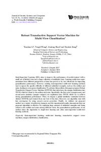
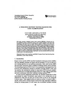
where φ (Χ ) denotes the nonlinear regression of forecasting results created by m methods denoted by ϕi (i = 1,2, L , m ) . However, constructing effective nonlinear combination function φ (Χ ) is very difficult because there is no fixed formula to use. 2.3 Principle of SVM Originally SVM was used for classification, i.e. searching for the optimal separating surface, the hyperplane, equidistant from the two classes (Vapnik 1995). This optimal separating hyperplane has many nice statistical properties. SVC is outlined first for the linearly separable case. Kernel functions are then introduced in order to construct non-linear decision surfaces. Finally, for noisy data, when complete separation of the two classes may not be desirable, slack variables are introduced to allow for training errors. The Support Vector Methods can also be applied to the case of regression by introducing an ε -insensitive loss function (Vapnik 1995 ; Smola 1996). As with the Support Vector Classification algorithm, optimal separating hyperplane is searched for regression. Support Vector Regression (SVR) relied on defining a loss function that ignored errors that were within a certain distance of the true value. Moreover, loss function allows the concepts of margin to be carried over to the regression case keeping all of the nice statistical properties. SVR also results in a quadratic programming. In two dimensions space the optimal separating hyperplanes for SVC and SVR is shown in Figure 4.
x2
x2
Hy perplane
Hy perplane
Support Vector
Suppor t Vec tor
x1
x1
Fig. 4. The optimal separating hyperplanes for SVC (left) and SVR (right) Support vector regression (SVR) is a powerful technique to solve the nonlinear regression problem. There are several attractive characteristics of the SVR: robustness of the solution, sparseness of the regression, automatic control of the solutions complexity, good generalization performance (estimation accuracy) (Kanevski et al 2000, Kanevski 2004). Detailed descriptions of SVR can be found in Vapnik (Vapnik 1995) and Smola (Smola 1996). 2.4 Nonlinear Spatio-Temporal Regression by SVM Suppose there are two forecasts such as temporal forecasting fT and. spatial forecasting f S . The question is how to combine these different forecasts into a signal forecasting yˆ , which is assumed to be a more accurate forecasting. In fact, a nonlinear combination forecasting model can be viewed as nonlinear information processing system which can be represented as: (4) yˆ = φ( X ) = φ( fT , f S ),
where X is attribute vector, which consists of fT and f S , and φ ( X ) is a nonlinear prediction function, which is used to predict the value of y knowing individual temporal forecasting fT and. spatial forecasting f S . Thus, the nonlinear combination function can be formulated in the following form: N
φ( fT , f S ) = ∑ (ai* − α i ) K (( fT , f S )' , ( fT , f S )),
(5)
i =1
where α i or α i* with non-zero is regarded as the "support vector (SV)" of the nonlinear prediction function; K (⋅,⋅) is kernel function. Usually we have more than one kernel to map the input space into feature space. Polynomial and RBF kernel functions are most common. Polynomial kernel function is defined as: K ( X ' , X " ) = ( X ' ⋅ X " + 1)d .
(6)
RBF kernel function is defined as: K ( X , X ) = exp(− '
"
X' − X" 2σ2
2
)
. (7) The question is which kernel functions provide good generalization for a particular problem. We could not say that one kernel outperforms the others. Therefore, one has to use more than one kernel functions for a particular problem. Some validation techniques such as bootstrapping and cross-validation can be used to determine a good kernel (Smola 1996). For instance, RBF has a parameter σ and one has to decide the value of σ before the experiment. Therefore, selection of this parameter is very important in order to achieve the expected accuracy. Therefore, a nonlinear regression function φ ( fT , f S ) is constructed by performing the SVR on the temporal forecasts fT and the spatial forecasts f S to find out the best spatiotemporal forecasting values.
3. Case study Experimental data sets are based on the annual air temperature at 26 meteorological stations provided by national meteorological center of P. R. China. The meteorological data between 1951 and 1992 are chosen as the training dataset for the forecasting the average temperature (degree/year) at Guangzhou city between 1993 and 2002. In the experiment, ARIMA (Auto-Regression in Moving Average) provided by Matlab software package is used for temporal forecasting, a dynamic recurrent neural network (Elman network) is applied for spatial forecasting (Cheng and Wang 2006;2007). Support vector regression is employed to find nonlinear combination function φ ( fT , f S ) (to generate the overall forecasting) (see Equation 5), the selection of the kernel function and corresponding parameters plays a significant role in obtaining good forecasting. In this study, polynomial function of degree d (see Equation 6), and radial basis function with radius σ (see Equation 7) has been tested. Table 1 shows the results of accuracy comparison between polynomial kernel and RBF kernel. Comparison of NMSE index and numbers of SVs indicates RBF kernel was more suitable for spatio-temporal forecasting. In addition, C also is a very important parameter, which controls the trade-off between maximizing the margin and minimizing the training error Kernel parameters, as well as C , are usually tuned by minimizing cross-validation or the testing error calculated on an independent set. Finally, RBF kernel is selected based on testing results with the kernel parameters σ =1, ε =0.001 and C =1000.
Table 1. A comparison of different kernels (C = 1000, ε = 0.001) Kernel
Group 1 Training NMSE 0.546 0.440 0.364 0.312 0.305 0.105 0.212 0.369
Polynomial (d=6) Polynomial (d=7) Polynomial (d=8) Polynomial (d=9) RBF ( σ = 0.5 ) RBF ( σ = 1 ) RBF ( σ = 1.5 ) RBF ( σ = 2 )
Numbers of SVs
42 41 40 41 42 39 41 42
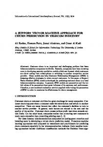
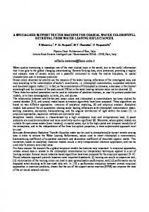
For comparison purposes, we also construct three other forecasting models, a pure time series model (ARIMA) for temporal forecasting, a pure Elman RNN (RNN) for spatial forecasting, and an improved STIFF (ISTIFF, which uses a linear regression of ARIMA and RNN, Cheng and Wang 2006), and compare them with the proposed model side by side in this study. The result forecasting plots and tables are shown in the subsequent Figure 5 and Table 2.
Annual average temperature(degree/year)
24 REAL
RNN
ARIMA
ISTIFF
SVM
22
20
18 1993
1995
1997
1999
2001 YEAR
Figure 5 Forecasting results by different methods Table 2: Comparison of forecasting accuracies Model Data Training data Testing data NMSE Rank NMSE Rank RNN 0.632 4 0.864 4 ARIMA 0.386 3 0.415 3 ISTIFF 0.207 2 0.268 2 SVM 0.105 1 0.193 1 From Figure 5 and Table 2, we can see that the SVM based nonlinear regression achieved better forecasting accuracy than linear combination of spatio-temporal forecasting
(ISTIFF), which is better than pure time series model for temporal forecasting, and pure Elman RNN for spatial forecasting respectively.
4. Conclusion In this study, a support vector regression algorithm is introduced to construct and find out nonlinear combination functions related to the spatial and temporal dimensions. The forecasting results show that nonlinear integrated spatio-temporal forecasting model using support vector regression obtains better forecasting accuracy than linear combination of spatio-temporal forecasting. Further studies are needed to extend the nonlinear spatiotemporal regression to address spatio-temporal forecasting involving multiple variables.
Acknowledgements The research is supported by the Major State Basic Research Development Program of China (973 Program, No. 2006CB701306) and the Ministry of Education of China (985 Project, No. 105203200400006).
5. References Cheng T and Wang J, 2006, Applications of spatio-temporal data mining and knowledge for forest fire. ISPRS Technical Commission VII Mid Term Symposium, Enschede, 148- 53. Cheng T and Wang J, 2007, Application of a dynamic recurrent neural network in spatio-temporal forecasting. to be presented to International Workshop on Information Fusion and Geographical Information Systems (IF&GIS-07), May 27-29, St. Petersburg. Cressie N and Majure J.J, 1997, Spatio-temporal statistical modelling of livestock waste in streams. Journal of Agricultural, Biological and Environmental Statistics, 2(5):20-28. Deutsch S.J and Ramos J.A, 1986, Space-time modelling of vector hydrologic sequences. Water Resources Bulletin, 22(6):967-980. Dong J, 2000a, A new nonlinear combination forecasting method based on fuzzy model and its application. System engineering: Theory & Practice, 5:109-114. Dong J, 2000b, Research on nonlinear combination forecasting method based on wavelet network. Journal of Systems Engineering, 15(4): 383-388. Pfeifer P.E and Deutsch S.J, 1990, A statima model-building procedure with application to description and regional forecasting. Journal of Forecasting, 9:50-59. Pokrajac D and Obradovic Z, 2001, Improved spatial-temporal forecasting through modelling of spatial residuals in recent history. Proceedings of first international SIAM conference on data-mining, Chicago, 368-386. Jiang L and Xie X.Y, 1999, A new nonlinear compound forecasting method based on ANN. Journal of Xi’an Institute of post and telecommunication, 4(1): 37-41. Kanevski M, Wong P and Canu S, 2000, Spatial Data Mapping with Support Vector Regression and Geostatistics. 7th International Conference on Neural Information Processing, Taepon, Korea. Nov. 14-18, 1307-1311. Kanevski M et al, 2004, Environmental data mining and modelling based on machine learning algorithms and geostatistics. Journal of Environmental Modelling and Software, 19:845-855. Smola A.J, 1996, Regression estimation with support vector learning machines. Master's thesis, Technische Universitot Miinchen. Vapnik V, 1995, The nature of statistical learning theory. Sprinner-Verlag, New York. Wang L.P, 2005, Support Vector Machines: Theory and Application, Springer, Berlin. Wang L.P and Fu X.J, 2005, Data Mining with Computational Intelligence, Springer, Berlin. Wen X and Niu M, 1994, A new nonlinear combination forecasting method based on neural network. System engineering: Theory & Practice, 14(12): 66-72.