Interface-capturing methods for two-phase flows - Stanford University

117

Center for Turbulence Research Annual Research Briefs 2017

Interface-capturing methods for two-phase flows: An overview and recent developments By S. Mirjalili, S. S. Jain

AND

M. S. Dodd

1. Motivation and objectives Two-phase flows are of great interest in natural and industrial applications such as rain formation (Shaw 2003), breaking waves (Melville 1996), spray atomization (Sirignano 1999) and bubbly flows (Sato et al. 1981; Clift et al. 2005). The purpose of this report is to survey the available interface-capturing methods for two-phase flows and to present them in a consistent fashion to facilitate comparison. We highlight the outstanding issues and challenges in two-phase flow modeling and discuss the relative advantages and disadvantages of the various interface-capturing methodologies. The literature on these methods continues to grow in an almost intractable manner. Hence, we will focus on interface-capturing methodologies that are currently in use and being actively developed by the two-phase community. Moreover, within different categories, we will only chronologically review milestones while alluding to the state of the art or most promising research directions. We apologize beforehand if we have overseen major contributions. Hopefully, this work can serve as an update/overview to veterans of the two-phase community while also guiding new researchers of the field in choosing a two-phase flow solver best suited for their applications. All conclusions and recommendations in this work are qualitative; quantitative comparison between different two-phase flow categories or methods would be complementary to this work.

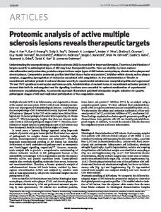
2. Overview and challenges Within the computational modeling community, problems involving two fluid phases are referred to as two-phase flows; whereas, multiphase flows consist of a broader category of problems including particle-laden flows. For the scope of this report, we will only concern ourselves with immiscible two-phase flows. While analytical studies of such flows date back to the 19th century (e.g., Plateau 1873), the scope of analytical work, even for the simplest problems, is often very limited. Experimental observations of realistic applications are also very difficult, as many of the experimental techniques cannot be extended to two-phase flows (Prosperetti & Tryggvason 2009). This motivates the development of accurate, physically consistent and cost-effective numerical methods for capturing the interface and coupling it to the momentum conservation equation. Unfortunately, constructing such methods is a difficult task given the challenges presented by two-phase flows. These challenges include, but are not limited to (1) enforcing mass, momentum and kinetic energy conservation, (2) modeling discontinuities in properties across the interface, especially large jumps in density, (3) handling complex topologies and separation of scales, (4) achieving robustness for simulation of realistic flows, (5) accurately implementing surface tension forces. Different two-phase modeling classes and their prominent methods are demonstrated in Figure 1, where we have highlighted with ellipses the classes and methods that are

118

Mirjalili, Jain & Dodd

currently of most interest in the community and are examined in this work. In this Figure, diffuse-interface approaches are also distinguished from sharp-interface approaches by gray background colors. While two-fluid models are found to be applicable for simple problems, they have been found to be unsuitable for realistic scenarios (Prosperetti & Tryggvason 2009). We refer the reader to Ishii & Hibiki (2010) and Prosperetti & Tryggvason (2009) for comprehensive discussions on two-fluid models. Moreover, for those interested in marker-and-cell (MAC) and front-tracking methods, detailed discussions are presented in McKee et al. (2008) and Tryggvason et al. (2011) respectively. The lattice Boltzmann method (LBM), smoothed-particle hydrodynamics (SPH) and constrained interpolation profile (CIP) are also left out of this report. As one can see from Figure 1, the interface-capturing methods of choice for this work (ellipses in Figure 1) all belong to the one-fluid formulation of two-phase modeling approaches. These methods are the volume-of-fluid (VOF), level-set (LS) and phase-field (PF) methods. For these classes of methods, we will first introduce them and their different variants and then describe the most influential versions and seek to update the reader on the current status of each class. We refer the reader to Tryggvason et al. (2011) for an introduction to governing equations for two-phase flows in the one-fluid model. We will only consider incompressible flows herein. Before going through the interface-tracking methods, we should emphasize that in coupling any of the above methods with the momentum equation in nonconservative form 1 ∂u + ∇ · (u ⊗ u) = −∇P + ∇ · µ(∇u + ∇T u) + FST , (2.1) ∂t ρ or in conservative form, as in ∂(ρu) + ∇ · (ρu ⊗ u) = −∇P + ∇ · µ(∇u + ∇T u) + FST , (2.2) ∂t there are many considerations for modeling the surface tension force , FST . In addition, apart from how density and viscosity are calculated, some extra care must be taken for discretization of the momentum fluxes. We expand upon these rather fundamental notions in the following section.

3. Momentum equation discretization in one-fluid models Any interface-capturing method would be coupled to the momentum equation through the computation of local density, viscosity and surface tension forces. In sharp-interface approaches, the density and viscosity values experience a jump across the interface, while in diffuse-interface approaches, these scalar fields are functions (often linear) of the local phase indicator function. Surface tension forces can be discretely implemented as stresses or body forces, often known as integral and volumetric formulations respectively. An important requirement for two-phase flow solvers is the discrete balance of the surface tension and pressure gradient terms (Fran¸cois et al. 2006). Integral formulations have yet to achieve this requirement, but have the advantage of automatic momentum conservation (zero total force on a closed surface). On the other hand, volumetric formulations have been successful at attaining this discrete balance. All in all, a well-balanced, momentum-conserving surface tension force formulation does not currently exist (Popinet 2018). Generally speaking, the volumetric formulation has been much more popular within the existing literature.

A review of interface-capturing methods for two-phase flows

119

Two-phase flows

LBM

SPH

Two-fluid

One-fluid

Interface-tracking

classes

MAC

Geometric VOF

Split

Unsplit

Front-tracking

models

approaches

Interface-capturing

VOF

Algebraic VOF

Compressive

Level set

Phase field

CLSVOF

CLS

CIP

THINC

Figure 1. Classification of numerical methods for two-phase flows. The interface-capturing methods, covered in the present work, are marked by ellipses. Methods that use a sharp-interface approach have a white background while diffuse-interface approaches have a gray background. Abbreviations are defined in the main text.

Popinet (2018) observed that all well-known volumetric formulations, including the original continuous surface force (CSF, Brackbill et al. 1992), ghost-fluid method (GFM, Fedkiw et al. 1999) and smoothed Heaviside method (Sussman et al. 1994) can be written in the form FST = σκδs n, which is commonly known as the CSF formulation, where σ is the surface tension and δs is a numerical Dirac delta function specific to each method. Therefore, a critical component of different surface tension calculation methods is the accuracy of calculating the normal vector (n) and curvature (κ). A common approach has been to compute normal vectors from spatially differentiating a smooth field (sometimes by a smoothening kernel), and subsequently taking the divergence of the normal vectors to obtain curvatures. In some sharp interface approaches (e.g., VOF), a smooth field is not readily available. Therefore, in recent years many new codes using sharp-interface approaches have employed height-functions for more accurate estimation of normals and/or curvatures (Sussman & Ohta 2009; Popinet 2009; Owkes & Desjardins 2015; Ivey & Moin 2015). Although height-functions can be very attractive in terms of accuracy, convergence and momentum conservation properties, their accuracy and robustness suffers at low resolutions, specifically when κ∆x > 1/5 (Popinet 2018). Thus, robust implementation of these methods is not straightforward and entails a smooth transition to alternative techniques such as parabolic reconstruction of surface tension (PROST), introduced in Renardy & Renardy (2002). The PROST method has been extended to unstructured meshes by Evrard et al. (2017). Their method can be interpreted as a generalization of the height-function method, and it converges with the same order of accuracy as height-function techniques. However, to date, it has only been applied

120


to two-dimensional unstructured meshes due to additional challenges and complexity presented in three dimensions. A discussion on numerical implementation of surface tension is incomplete without the mention of spurious currents. These artificial flows can be detrimental in practical twophase flows, leading to artificial generation of kinetic energy and heat transfer (Hardt & Wondra 2008; Gupta et al. 2009). Accurate direct numerical simulation (DNS) of turbulent two-phase flows is only possible if the root-mean-squared (r.m.s.) velocity of the spurious currents is negligible relative to the velocity fluctuations due to turbulence, as demonstrated recently by Dodd & Ferrante (2016). Accurate curvature estimation and well-balanced surface tension force discretization are required for reducing spurious currents. A test case assessing the relative magnitude of these currents is therefore an essential benchmark for the evaluation of surface tension implementation. Often times, the magnitude of spurious currents in a static drop test case at a specific time is reported (originally due to Gunstensen 1992). However, improvements to this measure are necessary as shown by Magnini et al. (2016), for instance, by reporting the history or time-averaged norm of spurious currents. In addition, these authors suggest examining spurious currents for a moving drop. Finally, much progress has been made in recent years towards the goal of discrete conservation of energy for two-phase flows, particularly at high density ratios. For Cartesian staggered grids, a method that discretely conserves kinetic energy in the absence of viscous dissipation and surface tension forces was presented in Fuster (2013). In general, it is now well-established that for accurate and robust simulations at large density ratios, momentum should be transported conservatively via Eq. (2.2) and also consistently with respect to mass advection (Popinet 2009; Raessi & Pitsch 2012; Chenadec & Pitsch 2013; Ivey et al. 2016). This correction has been shown to significantly improve the energy conservation properties of two-phase flow solvers.

4. Volume-of-fluid method In the class of volume-of-fluid (VOF) methods, the phase indicator function, H(x, t), is defined as ( 1 if x is in the reference fluid, H(x, t) = (4.1) 0 if x is in the other fluid. In the absence of phase change, each fluid parcel retains its phase indicator value during its motion. Therefore, the material derivative of H is zero, i.e. ∂H DH = + ∇ · (uH) − H∇ · u = 0. Dt ∂t

(4.2)

The volume fraction is defined as the spatial average of the phase indicator function (H) in each computational cell (Ω), Z 1 Ck (t) = H(x, t) dV, (4.3) V Ω where V is the volume of the k-th cell. We then integrate Eq. (4.2) over the computational cell and use the definition introduced in Eq. (4.3) to obtain Z Z ∂Ck (t) V + (u · n)H(x, t) dS = H∇ · u dV. (4.4) ∂t ∂Ω Ω


121

While in incompressible flows ∇ · u = 0, this term is retained in Eq. (4.4) for reasons related to numerical implementation that will be explained later. In geometric VOF methods an approximation to H is found geometrically (e.g., by a plane), whereas in algebraic VOF methods H is represented by a function (e.g., polynomial or trigonometric function). 4.1. Geometric VOF Geometric VOF methods proceed in two steps. First, the interface is reconstructed in each computational cell from the knowledge of the volume fraction field. Second, the reconstructed interface is advected by computing the fluxed volume across each computational cell using geometric methods. In the following, we review the state of the art for performing these two tasks. 4.1.1. Interface reconstruction For the first task, the most widely used method is the piecewise linear interface calculation (PLIC) scheme (Debar 1974). In this approach, the interface is approximated in each interfacial cell as a line in two dimensions or a plane in three dimensions as n · x + α = 0,

(4.5)

where α is the constant in the plane equation that is selected to enforce that the volume cut by the interface is equal to Ck in the computational cell. The main choice left to the user is how to compute the interface normal, n. Youngs’ method (Youngs 1982) estimates n as a normalized gradient of Ck . This method is fast and performs best at low resolutions, but at higher resolutions its accuracy decreases from second to first order. A method that performs better at high resolutions is the centered-columns method (Scardovelli & Zaleski 2003). An approach that combines the desirable properties at both low and high resolutions is the mixed Youngs-centered (MYC) method (Aulisa et al. 2007). Pilliod & Puckett (2004) introduced the efficient least-squares volume-of-fluid interface reconstruction algorithm (ELVIRA) method. On structured Cartesian meshes, this approach uses a least-squares error minimization to select between normal vector candidates. Its extension to three dimensional unstructured meshes is more complicated, but has been accomplished by Jofre et al. (2014). ELVIRA is second-order accurate but has high computational cost, especially in three dimensions due to an increased number of normal candidates. For unstructured meshes and general polyhedral cells, Ivey & Moin (2015) developed an embedded height-function framework to compute second-order accurate normals. On Cartesian meshes, the MYC method appears to be the preferred method because of its low cost and relatively high degree of accuracy on structured meshes, and as such, it has been implemented in several free softwares (e.g., Popinet 2012, 2013; Arrufat et al. 2014). On unstructured meshes, the favored method for computing interface normals is less clear. After the normal n has been calculated, the next task is to compute α. For right hexahedral cells, Scardovelli & Zaleski (2000) presented analytical methods for computing α. For general polyhedra, a root-finding algorithm is typically employed to find α, for which VOF-specific libraries exist, e.g., the VOFTools library by López et al. (2017). 4.1.2. Interface advection The interface is advected by integrating Eq. (4.4) in time. The main decision left to the user is on how the volume fluxes of the reference fluid are calculated. Two classes of advection algorithms have emerged: (i) split methods that rely on operator-splitting to perform

122


a series of one dimensional advections in each spatial dimension and (ii) unsplit methods, which advect the interface in one step. Split methods are algorithmically straightforward to implement compared to multidimensional (unsplit) schemes. Unsplit schemes involve computation of complex flux polyhedra in computational cells containing the interface. These computations are expensive and can lead to significant parallel load imbalance if left untreated (Jofre et al. 2015). On the other hand, unsplit methods have the advantage of only requiring one advection and reconstruction step and are more amenable for general three-dimensional unstructured meshes. In addition, Pilliod & Puckett (2004) showed that unsplit methods better resolve interfaces that are non-smooth (i.e. contain corners). How this increased resolution capability translates into practical applications (e.g., Prakash et al. 2016; Mortazavi et al. 2016) is an open question. As previously mentioned, split advection schemes use operator-splitting to decompose Eq. (4.4) into a series of one dimensional advections. Because terms like ∂u/∂x are generally non-zero, the right-hand side in Eq. (4.4) is retained. This is in contrast to unsplit schemes which omit the last term due incompressibility (∇·u). In two dimensions, the first split advection scheme to satisfy the boundedness condition, 0 ≤ Ck ≤ 1, and mass conservation in incompressible flow is known as the Eulerian implicit - Lagrangian explicit (EI-LE) scheme (Tryggvason et al. 2011). Aulisa et al. (2007) extended the EI-LE scheme to three dimensions by creating EILE-3D. EILE-3D uses a series of three EI-LE advection steps, one in each spatial direction. This discretely mass-conserving scheme satisfies the boundedness condition, but has the disadvantage of requiring six advection and interface reconstruction steps as well as the requirement to compute three twodimensional divergence-free velocity fields. Later, Weymouth & Yue (2010) developed a split advection scheme that consists of three Lagrangian explicit (LE) steps that are both bounded (0 ≤ Ck ≤ 1) and discretely conservative. The only drawback is that it introduces an additional CFL restriction to guarantee boundedness of Ck . However, this restriction is relatively benign. The Weymouth & Yue method is implemented in the free software Basilisk (Popinet 2013) and PARIS Simulator (Arrufat et al. 2014). Another method to extend the EI-LE advection scheme to three dimensions was given by Baraldi et al. (2014). This approach introduces an algebraic step in the third dimension that ensures mass is discretely conserved. The downside to this is that the algebraic step can produce overshoots (Ck > 1) or undershoots (Ck < 0), and therefore a redistribution algorithm is required to ensure boundedness. Further tests of the split advection schemes which include a cost comparison would be beneficial. Unsplit VOF advection methods compute and transport the fluxed volume in one step. Rider & Kothe (1998) proposed one of the first unsplit VOF advection schemes in the framework of PLIC interface reconstruction. Face centered velocity components were used to construct trapezoidal flux regions. These flux regions can potentially overlap, which can ultimately lead to the condition 0 ≤ Ck ≤ 1 not being satisfied exactly. L´ opez et al. (2004) developed a two-dimensional unsplit geometric advection scheme which used cell vertex velocities instead of edge velocities. This change resulted in no overlap of flux regions which improved the mass conservation compared to Rider & Kothe (1998). Owkes & Desjardins (2014) extended the work of López et al. (2004), yielding a bounded, mass-conserving three-dimensional unsplit VOF advection algorithm. Their scheme addressed outstanding conservation issues in three-dimensional unsplit methods, namely how to address flux hexahedra that overlap during the advection step. Jofre et al. (2014) extended the work of Owkes & Desjardins (2014) to unstructured meshes and non-convex polyhedra. Ivey & Moin (2017) further advanced the computation of


123

flux polyhedra on unstructured meshes to yield a discretely conservative and bounded unsplit advection scheme. It should be noted that all the state of the art unsplit VOF advection methods use cell vertex velocities to form the flux polyhedra as opposed to edge velocities. A possible departure from this framework is given by Roenby et al. (2016). Although the performance and accuracy of this method has not yet been compared to conventional geometric VOF methods, it offers a potentially more cost-effective approach to VOF advection on unstructured meshes because it does not require PLIC interface reconstruction and complex geometric computations of flux volumes. It is important to note that in VOF advection schemes, discrete mass conservation is only guaranteed if ∇ · u = 0 is satisfied discretely in every grid cell. In practice, the condition ∇ · u = 0 is typically only satisfied up to some user-specified tolerance through the iterative solution of the Poisson equation for pressure. To obtain discrete conservation of mass to machine precision in every grid cell cost effectively, the Poisson equation should be solved directly instead of iteratively (Dodd & Ferrante 2014). 4.2. Algebraic VOF Algebraic VOF (AVOF) methods are probably one of the oldest classes of interfacecapturing methods and the first of the VOF-type methods (Hirt & Nichols 1981). In these methods, the volume fraction, C, is obtained via Eq. (4.4) with a numerical approximation (volume-averaged, polynomial or hyperbolic-tangent representation) for the phase indicator function, H. These methods compute the fluxes algebraically without the need for geometric reconstruction of the interface, hence the name. Broadly, algebraic VOF methods can be classified into two categories based on the approach used to compute the fluxes, (a) compressive class and (b) THINC class (tangent of hyperbola for interface capturing). 4.2.1. Compressive schemes Compressive schemes use the information of the orientation of the interface (interface normal) with respect to the cell face and compute the face flux, Ff , for the VOF function as Ff = γ(θ)FHRS + [1 − γ(θ)] FHDS ,

(4.6)

where FHRS is the flux computed using a high-resolution scheme and FHDS is the flux computed using a high-order downwinding scheme, γ is a blending function and θ is the angle between the cell face normal and the interface normal – defining the orientation of the interface with respect to the cell face. To expand on this, when computing fluxes across each face, if the interface normal is aligned along the cell face normal, a HDS scheme is used, whereas when the interface normal is perpendicular to the cell face normal a HRS scheme is used and for all the intermediate situations a combination of these two schemes is employed depending on the choice of the blending function. Among various compressive methods such as high resolution interface capturing scheme (HRIC) (Muzaferija et al. 1998), compressive interface capturing scheme for arbitrary meshes (CICSAM) (Ubbink & Issa 1999), switching technique for advection and capturing of surfaces (STACS) (Darwish & Moukalled 2006), high-resolution artificial compressive formulation (HiRAC) (Heyns et al. 2013) and modified-CICSAM (M-CICSAM), M-CICSAM is better than HRIC, STACS and CICSAM (Zhang et al. 2014), whereas a comparison between HiRAC and M-CICSAM is yet to be made. Unfortunately, the accuracy of compressive algebraic VOF methods is generally found to be about an order of magnitude lower than the state of the art geometric VOF methods, and is also found to depend on the local cell

124


Courant number. Additionally, to avoid the diffusion of the interface when the interface gets deformed in flows with high strain rates, an artificial interface sharpening term is typically added to the right-hand side of Eq. (4.4). 4.2.2. THINC schemes THINC schemes (Xiao et al. 2005) are a group of relatively new methods within algebraic VOF where a hyperbolic-tangent profile is assumed for the phase indicator function (H) within the cell containing the interface, and the fluxes are computed algebraically according to this assumption from Eq. (4.4). According to claims by Xie et al. (2014), the accuracy of these methods can be close to geometric VOF methods at lesser cost. Hence, THINC schemes are gaining popularity these days. Moreover, unlike the compressive schemes introduced in Section 4.2.1, these methods do not require artificial compression and are independent of the local cell Courant number. However, more rigorous studies on the comparison of the cost of these methods in three-dimensions - UMTHINC (Ii et al. 2014; Xie et al. 2014) against the state of the art geometric VOF methods are warranted. Flux limiters, such as the multidimensional universal limiter with explicit solution (MULES) can also be used to advect the color function algebraically, but the accuracy of these methods is not on par with either the THINC class or the latest compressive class methods (Roenby et al. 2016). Overall, the performance of all the algebraic VOF methods have yet to be rigorously tested for large-scale realistic simulations.

5. Level-set methods Level set methods were first developed and used in the context of computer graphics and image processing (Sethian 1999). They were extended to the case of two-phase flows by Sussman et al. (1994). A traditional level set function is a signed-distance function φ(x, t), that represents the shortest distance to the interface. These methods solve the advection equation ∂φ + u · n|∇φ| = 0, (5.1) ∂t to update φ at every time step and are commonly discretized with a Hamilton-Jacobi weighted essentially non-oscillating (HJ-WENO) type scheme in space and a total variation diminishing Runge-Kutta (TVD-RK) scheme in time. Sadly, φ loses its signeddistance property after the advection step, and hence needs to be reinitialized. Level set methods offer many advantages over other methods such as: (1) accurate computation of normals and curvature using n = ∇φ/|∇φ| and κ = ∇ · n, due to smoothness of the φ field and (2) straightforward extensions to Cartesian adaptive mesh refinement (AMR). However, the biggest disadvantage of these methods is the fact that mass of each phase is not conserved, a crucial requirement for numerical modeling of realistic two-phase flows. While there are multiple fixes to limit the mass loss as described in Section 5.2, this problem cannot be eliminated completely. 5.1. Reinitialization The conventional approach to reinitialize φ is to compute the interface location (φ = 0) and to recompute the distance to the interface at all other points. However, this method was found to be too expensive with a complexity of O(N 3 ) and was found to distort the interface. Hence, Sussman et al. (1994) proposed a PDE based reinitialization method φτ = sgn(φ0 )(|∇φ| − 1) = 0,

(5.2)


125

where sgn is a smoothed signum function. Reinitialization of φ can also be performed by solving the Eikonal equation of the form ||∇φ|| = 1.

(5.3)

Fast numerical methods such as the fast-marching method (FMM) (Chopp 2001) and the fast-sweeping method (FSM) (Zhao 2005) have been developed to solve this equation. FMM uses a heap structure to store and order the grid points where the Eikonal equation is solved and has a complexity of O(N log N ), whereas the FSM uses Gauss-Seidel iterations with alternating sweeping orderings and hence the number of sweeps is bounded: 2n for Rn with a complexity of O(N ). These methods seem attractive due to their low cost and reduced mass-loss error with the use of higher-order extensions; however, there is an inherent difficulty in scalable parallel implementation of these methods due to loadbalancing issues and the requirement of high number of iterations in the regions where the characteristics cross the sub-domain multiple times. 5.2. Mass-loss corrections The PDE based reinitialization method proposed by Sussman et al. (1994) was found to move the interface location (φ = 0) significantly, resulting in mass loss. Russo & Smereka (2000) came up with a sub-cell fix, wherein they used the location of the interface in computing the fluxes with second-order accuracy for cells containing the interface. This approach was further extended to fourth-order accuracy by du Chéné et al. (2008). In a different approach, Enright et al. (2002) proposed a hybrid particle level set method (HPLS), wherein they seed the interface with particles, and employ algorithms to attract them towards the interface and to correct φ when the particles cross the interface. With this approach, they found that the mass loss reduced from 80% to 2.6% for the case of a three-dimensional drop in shear flow. Some researchers have also successfully taken advantage of the fact that the mass conservation error reduces with mesh refinement. For instance, Herrmann (2008) solves the level-set equations on an auxiliary high-resolution grid, while Gibou et al. (2018) highly refine the regions close to the interface via AMR. While these methods successfully reduce the mass-loss error, the simplicity of the level-set method is generally lost, and they still do not achieve discrete mass conservation. Hence, level-set methods based on the signed-distance function are becoming less popular in the two-phase community compared to other mass-conserving methods. Nevertheless, the numerical tools developed for these methods, such as FMM and FSM, are being actively employed within other classes of methods (see Section 5.3). 5.3. Conservative level-set method In an attempt to tackle the conservation issues of the level-set method, the conservative level-set method was introduced by Olsson & Kreiss (2005), replacing the sharp interface between two immiscible phases with a diffuse profile that takes the form of s(x) , (5.4) φ(x) = 0.5 1 + tanh 2 where x is the position, s(x) is the signed distance function, controls the interface thickness, and φ varies from 0 to 1. In that seminal paper, φ is advected as ∂φ + ∇ · (uφ) = 0. ∂t

(5.5)

126


Afterwards, the reinitialization step, defined as ∂φ = ∇ · [∇φ − φ(1 − φ)n] , ∂τ

(5.6)

is integrated in pseudo-time, τ , till convergence, where n = ∇φτ =0 / |∇φτ =0 | and secondorder central-differences are used for all spatial derivatives. The advection and reinitialization steps are coupled to a momentum transport step where density and viscosity are linear functions of φ, and surface tension is computed in a CSF formulation. Compared to volume-of-fluid and traditional level-set methods, this mass-conserving scheme is easy to implement and an extension to unstructured three-dimensional grids can be found in Balczar et al. (2014). In Olsson et al. (2007), the reinitialization equation is modified by projecting the diffusive flux in the normal direction, ∂φ = ∇ · {[(∇φ · n) − φ(1 − φ)] n} , ∂τ

(5.7)

which reduces the errors brought by tangential fluxes during reinitialization using Eq. (5.6). These equations, which are commonly referred to as the original conservative level-set R method, are mass conserving as V φdV is conserved. Moreover, straightforward computation of the normal and curvature values is possible due to the smooth nature of φ. However, the numerical solution of Eq. (5.7) is susceptible to dispersion errors. Thus, in order to restrict oscillations in the normal vector and keep φ bounded, TVD schemes have to be employed which result in numerical dissipation. Moreover, high levels of reinitialization using Eq. (5.7) have been shown to result in artificial deformation of the interface, even if the normal vector is exact (McCaslin & Desjardins 2014). Waclawczyk (2015) rectified this issue by taking advantage of the distance level set to find a reinitialization equation consistent with the traditional level-set reinitialization equation, Eq. (5.2), as ∂φ = ∇ · [φ(1 − φ)(|∇φmap · n| − 1)n], ∂τ

(5.8)

where φmap = ln(φ/(1 − φ)) is the distance level-set function and the normal vector is n = ∇φmap,τ =0 / ∇φmap,τ =0 . This approach still requires TVD advection for robustness. Chiodi & Desjardins (2017) recently combined the reinitialization equation of Waclawczyk (2015) with the accurate conservative level-set (ACLS) method introduced first in Desjardins et al. (2008). They reformulated the reinitialization equation in a form that remains conservative and is not subject to large errors at high levels of reinitialization while allowing for non-TVD high-order transport of φ. This is possible by computing the normal vectors from the reconstructed level-set function, obtained using FMM (as in Desjardins et al. 2008). Furthermore, they modify the reinitialization equation in the form ∂φ 1 =∇· (|∇φmap · n| − 1)n , (5.9) ∂τ 4cosh2 [φmap /(2)] to be insensitive to the bounds of φ. Chiodi & Desjardins (2017) follows the ACLS approach by using a sharp description of the interface, hence also incurring mass conservation errors which are albeit much smaller than traditional level-set schemes. Moreover, based on run-times reported for a two-phase jet calculation, the cost of Chiodi & Desjardins (2017) is much larger than the original CLS schemes. Finally, we should emphasize that in the continuous limit, the right-hand side of Eqs. (5.6) – (5.9) do not displace the φ = 0.5 contour which represents the interface. This is a necessary requirement for any valid reinitialization technique.


127

6. Phase-field methods The hyperbolic tangent shape of the interface in conservative level-set methods, Eq. (5.4), resembles the thermodynamically derived equilibrium profile in phase-field methods. In this class of methods, the transport equation governing the phase indicator is modified by incorporating physical effects that govern thin interfaces. Although in realistic immiscible two-phase flow applications, the physical thickness of the interface is practically impossible to resolve numerically, these methods offer some desirable properties that have attracted the interest of two-phase flow modelers in recent years (Anderson et al. 1998; Badalassi et al. 2003; Ding et al. 2007). Traditionally, phase-field methods were either based on the Cahn-Hilliard or the Allen-Cahn equations, which are two important gradient flows of the Ginzburg-Landau-Wilson free energy functional. In a bounded physical domain given by Ω, this energy functional is defined on the H 1 (Ω) space in the form Z Z 1 2 2 |∇φ| dV + W (φ)dV , (6.1) F : H 1 (Ω) → [0, ∞], F (φ) = 2 Ω Ω where φ = −1 and φ = +1 represent the pure phases and W (s) = (1 − s2 )2 /4 is the mathematically approximated double-well potential. The Allen-Cahn equation is essentially a convection-diffusion equation with a source term. There is a plethora of well-established numerical methods for solving such equations. This easy to implement second order PDE is widely used in material science applications where phase change occurs. This equation is in fact, the L2 (Ω) gradient flow of the energy functional defined in Eq. (6.1), ∂φ + ∇ · (uφ) = 2 ∇2 φ − W 0 (φ). (6.2) ∂t Clearly, this equation is in nonconservative form. Some authors have sought to rectify this by adding space and time varying Lagrange multipliers (Yang et al. 2006; Kim et al. 2014). However, the inherent lack of conservation of φ in the Allen-Cahn equation is a major limitation for immiscible two-phase flows. The Cahn-Hilliard equation is a more popular option within the two-phase flow community as it conserves total mass. This equation, given by ∂φ + ∇ · (uφ) = −∇2 2 ∇2 φ − W 0 (φ) , (6.3) ∂t is the H −1 (Ω) gradient flow of the energy functional defined in Eq. (6.1). For this specific phase-field method, Jacqmin (1999) shows how surface tension force can be defined such that total energy (kinetic energy plus surface energy) is only dissipated, causing spurious currents to vanish. Most papers on Cahn-Hilliard, including Jacqmin (1999), have focused on equal or low density ratios. Ding et al. (2007) laid the foundation for applying these equations to flows with large density ratios. Later, Shen & Yang (2010) extended the work by Jacqmin (1999) to non-unity density ratios by elaborating on how the momentum equation for Allen-Cahn and Cahn-Hilliard systems should be modified such that these phase-field systems admit discrete energy laws in which the total energy is non-increasing. Dong & Shen (2012) later used this framework and presented a spectral element based solver which was suitable for handling the fourth order spatial derivatives in Eq. (6.3). Despite the Cahn-Hilliard based phase-field system’s advantage of upper bounds on total energy which leads to robustness and stability, the artificial dissipation of total energy is undesirable, especially for realistic applications such as turbulent two-phase flows. Moreover, handling a fourth order spatial derivative is cumbersome. Finally, equilibrium

128


solutions can yield phase values other than 1 and -1 at pure phases, which is unacceptable for high density ratios (Yue et al. 2007). In Dong & Shen (2012), this issue was handled by clipping these out of bounds values. Some authors such as Li et al. (2016) and Wang et al. (2015) have instead added corrections terms to the right hand side of Eq. (6.3), but such artificial fixes come with a penalty. Namely, the modified phase-field equations in such methods are no longer gradient flows of an energy functional, and in addition, they do not admit discrete energy laws. Owing to the aforementioned intrinsic deficiencies, neither of the traditional phase-field equations, Eqs. (6.2) and (6.3), are particularly suitable for simulation of immiscible twophase flows. This has motivated researchers to try to combine the advantages of the two equations while avoiding their issues. In Sun & Beckermann (2007), the curvature-driven flow in Allen-Cahn is subtracted out to obtain a second-order PDE suitable for twophase simulations. Later on, Chiu & Lin (2011) were inspired by the conservative-level-set literature to reformulate the phase field in Sun & Beckermann (2007) in a conservative form, giving ∇φ ∂φ + ∇ · (uφ) = γ∇ · ∇φ − φ(1 − φ) . (6.4) ∂t |∇φ| The right hand side in Eq. (6.4) is exactly the same as that used in the reinitialization step of the original conservative level-set method, Eq. (5.6). In spite of a dispersionrelation-preserving upwind scheme specially developed for the convection-diffusion equation, the authors could not guarantee the boundedness of φ and had to resort to massredistribution to handle overshoots and undershoots. In Mirjalili et al. (2017), they proved that with the same central-difference discretization used in the reinitialization step of CLS (Olsson & Kreiss 2005), one can choose the free parameters, and γ such that the boundedness of φ in Eq. (6.4) is automatically preserved. As a result, their second-order accurate, conservative and bounded phase-field method, when coupled to a momentum transport step with CSF for surface tension force, presents a easy-to-implement approach for two-phase modeling. Mirjalili et al. (2016) compares this solver with a state of the art two-phase solver based on unsplit geometric VOF. At the same resolution, the VOF method is more accurate than the phase-field method. However, at the same cost levels (CPU time), this phase-field method can actually produce similar accuracy levels as the VOF method. Based on their results, they also recommended that in lieu of using VOF at low resolutions, it is possible to achieve more accuracy at lower overall cost using a phase field with higher spatial resolution. Indeed, this idea has already been exploited in a hybrid phase field-VOF scheme presented in Liu & Yu (2016). Lastly, we would like to highlight an important shortcoming in the literature of phase-field methods. Many new methods are being regularly introduced to the community; however, phase-field methods have seldom been applied to realistic industrial/atmospheric two-phase problems. Such attempts are necessary and would further enlighten researchers and CFD users on the appropriateness of these methods.

7. Hybrid methods There are various hybrid methods available in the literature, such as coupled-levelset and volume-of-fluid method (CLSVOF) (Sussman & Puckett 2000), front-tracking coupled with VOF (Aulisa et al. 2007), and phase field coupled with VOF (Liu & Yu 2016). Of all these methods, CLSVOF has been quite successful since it takes advantage of level-sets in accurate computation of normals and curvature, and also improves


method

129

GVOF AVOF LS CLSVOF CLS PF

mass conservation momentum and kinetic-energy conservation ease of programming normals and curvature cost and scalability unstructured Meshes overall accuracy

33 3 3 3 3 33 33

33 7 3 3 33 33 3

3 7 3 33 3 3 3

33 3 7 33 7 3 33

overall potential

33

3

7

3

33 33 3 3 3 33 3 3 33 33 3 3 3 3 3

33

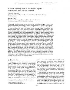
Table 1. Status of different interface-capturing methods: geometric volume of fluid (GVOF), algebraic volume of fluid (AVOF), level set (LS), coupled level set and volume of fluid (CLSVOF), conservative level set (CLS), and phase field (PF). Signs denote 33: good/solved, 3: satisfactory progress, 7: poor/no progress.

mass conservation by utilizing the VOF framework. There have been a few variations of CLSVOF that achieve discrete mass conservation (e.g. Tomar et al. 2005). Overall, the accuracy of this method is typically higher than a level-set or a VOF method, although the cost is also higher. This method also has issues in achieving parallel scalability due to the inherent difficulty in achieving balanced loads in the presence of operations required for both VOF and level-set methods.

8. Concluding remarks In this report, we have provided an overview of the most popular interface-capturing methods, with emphasis on modern developments. In the spirit of comparison, we have summarized the status of these methods in Table 1. The reader should be able to extract the rationale behind the ratings in this table from discussions presented in Sections 4-7. We found that the biggest challenge remaining in the field is in developing mass, momentum and total energy conserving schemes with reasonable cost and scalability (see Table 1). Indeed, these are required for realistic simulations of two-phase flows, especially in turbulent conditions. Moreover, by considering other relevant factors, particularly accuracy and modular adaptability to problems with practical significance (including compressible flows, unstructured meshes, scalar transport, and surfactant transport), we conclude in Table 1 that VOF and phase-field methods can be considered the most promising classes for future investment. On a separate note, while reviewing the literature for this report, we observed a conspicuous scarcity of benchmarks and test-cases that could help to evaluate the performance of new schemes in problems and conditions pertinent to practical applications. Firstly, we recommend the design of several test cases at realistic non-dimensional numbers in which the accuracy and robustness of the fully coupled solver (interface capturing scheme and momentum equation implementation) can be assessed. Secondly, when performing DNS or LES of two-phase turbulent flows, it is inevitable that some features (e.g., lig-

130


aments, films, and droplet fragments) are left under-resolved. It is important that the under-resolved features do not cause the numerical simulation to diverge or introduce artificial effects. Yet in papers introducing numerical methods we commonly see a focus on convergence rates and accuracy at rather high resolutions. Through assessment and presentation of the performance of solvers at low resolutions, this deficiency should also be addressed in future work. Hopefully, these improved benchmarks will motivate the emergence of methods that are more appropriate for tackling difficult, realistic problems in two-phase flows. As a final remark, we believe that additional work on multi-physics aspects of two-phase flows would be beneficial. A number of engineering applications require consideration of complex phenomena beyond the purely capillary effects reviewed here. For instance, the utilization of electrostatic effects in spray atomizers represents an interesting method to control the atomization of liquids (Gomez & Tang 1994; Tang & Gomez 1994; de la Mora 2007). Similarly, the interaction of acoustic waves with droplets, bubbles and interfaces in general is a problem of relevance for the acoustic traceability of ships in ocean (Trevorrow et al. 1994), for biomedical applications (Adami et al. 2016), and for fuel atomization in jet engines (Gajan et al. 2016) and hydrocarbon-fueled scramjets (Urzay 2017). The treatment of these advanced problems is in its infancy and requires creative extensions of the existing frameworks reviewed in this report.

Acknowledgments This investigation was funded by ONR, Grant #N00014-15-1-2726.

REFERENCES

Adami, S., Kaiser, J., Adams, N. & Bermejo-Moreno, I. 2016 Numerical modeling of shock waves in biomedicine. Proceedings of the Summer Program, Center for Turbulence Research, Stanford University, pp. 15–24. Anderson, D., McFadden, G. & Wheeler, A. 1998 Diffuse-interface methods in fluid mechanics. Annu. Rev. Fluid Mech. 30, 139–165. Arrufat, T. J., Dabiri, S., Fuster, D., Ling, Y., Malan, L., Scardovelli, R., Tryggvason, G., Yecko, P. & Zaleski, S. 2014 The PARIS-Simulator code. http://www.ida.upmc.fr/∼zaleski/paris/index.html. Aulisa, E., Manservisi, S., Scardovelli, R. & Zaleski, S. 2007 Interface reconstruction with least-squares fit and split advection in three-dimensional cartesian geometry. J. Comput. Phys. 225, 2301–2319. Badalassi, V., Ceniceros, H. & Banerjee, S. 2003 Computation of multiphase systems with phase field models. J. Comput. Phys. 190, 371–397. Balczar, N., Jofre, L., Lehmkuhl, O., Castro, J. & Rigola, J. 2014 A finitevolume/level-set method for simulating two-phase flows on unstructured grids. Int. J. Multiphase Flow 64, 55–72. Baraldi, A., Dodd, M. & Ferrante, A. 2014 A mass-conserving volume-of-fluid method: volume tracking and droplet surface-tension in incompressible isotropic turbulence. Comput. Fluids 96, 322–337. Brackbill, J., Kothe, D. & Zemach, C. 1992 A continuum method for modeling surface tension. J. Comput. Phys. 100, 335–354. Chenadec, V. L. & Pitsch, H. 2013 A monotonicity preserving conservative sharp


131

interface flow solver for high density ratio two-phase flows. J. Comput. Phys. 249, 185–203. ´ ne ´, A., Min, C. & Gibou, F. 2008 Second-order accurate computation of du Che curvatures in a level set framework using novel high-order reinitialization schemes. J. Sci. Comput. 35, 114–131. Chiodi, R. & Desjardins, O. 2017 A reformulation of the conservative level set reinitialization equation for accurate and robust simulation of complex multiphase flows. J. Comput. Phys. 343, 186–200. Chiu, P. H. & Lin, Y. T. 2011 A conservative phase field method for solving incompressible two-phase flows. J. Comput. Phys. pp. 185–204. Chopp, D. L. 2001 Some improvements of the fast marching method. SIAM J. Sci. Comput. 23, 230–244. Clift, R., Grace, J. R. & Weber, M. E. 2005 Bubbles, Drops, and Particles. Courier Corporation. Darwish, M. & Moukalled, F. 2006 Convective schemes for capturing interfaces of free-surface flows on unstructured grids. Numer. Heat Tr. B-Fund. 49, 19–42. Debar, R. 1974 Fundamentals of the KRAKEN code. LLNL Tech. Rep. #UCIR-760. Desjardins, O., Moureau, V. & Pitsch, H. 2008 An accurate conservative level set/ghost fluid method for simulating turbulent atomization. J. Comput. Phys. 227, 8395–8416. Ding, H., Spelt, P. D. & Shu, C. 2007 Diffuse interface model for incompressible two-phase flows with large density ratios. J. Comput. Phys. 226, 2078–2095. Dodd, M. S. & Ferrante, A. 2014 A fast pressure-correction method for incompressible two-fluid flows. J. Comput. Phys. 273, 416–434. Dodd, M. S. & Ferrante, A. 2016 On the interaction of Taylor length scale size droplets and isotropic turbulence. J. Fluid Mech. 806, 356–412. Dong, S. & Shen, J. 2012 A time-stepping scheme involving constant coefficient matrices for phase-field simulations of two-phase incompressible flows with large density ratios. J. Comput. Phys. 231, 5788–5804. Enright, D., Fedkiw, R., Ferziger, J. & Mitchell, I. 2002 A hybrid particle level set method for improved interface capturing. J. Comput. Phys. 183, 83–116. Evrard, F., Denner, F. & van Wachem, B. 2017 Estimation of curvature from volume fractions using parabolic reconstruction on two-dimensional unstructured meshes. J. Comput. Phys. 351, 271–294. Fedkiw, R. P., Aslam, T., Merriman, B. & Osher, S. 1999 A non-oscillatory Eulerian approach to interfaces in multimaterial flows (the ghost fluid method). J. Comput. Phys. 152, 457–492. ´ ndez. de la Mora, J. 2007 The fluid dynamics of Taylor cones. Annu. Rev. Ferna Fluid Mech. 39, 217–243. Franc ¸ ois, M. M., Cummins, S. J., Dendy, E. D., Kothe, D. B., Sicilian, J. M. & Williams, M. W. 2006 A balanced-force algorithm for continuous and sharp interfacial surface tension models within a volume tracking framework. J. Comput. Phys. 213, 141–173. Fuster, D. 2013 An energy preserving formulation for the simulation of multiphase turbulent flows. J. Comput. Phys. 235, 114–128. Gajan, P., Simon, F., Orain, M. & Bodoc, V. 2016 Investigation and modeling of combustion instabilities in aero engines. AerospaceLab AL11–09.

132


Gibou, F., Fedkiw, R. & Osher, S. 2018 A review of level-set methods and some recent applications. J. Comput. Phys. 353, 82–109. Gomez, A. & Tang, K. 1994 Charge and fission of droplets in electrostatic sprays. Phys. Fluids 6, 404–414. Gunstensen, A. K. 1992 Lattice-Boltzmann Studies of Multiphase Flow Through Porous Media. Ph.D. Thesis, MIT. Gupta, R., Fletcher, D. F. & Haynes, B. S. 2009 On the CFD modelling of Taylor flow in microchannels. Chem. Eng. Sci. 64, 2941–2950. Hardt, S. & Wondra, F. 2008 Evaporation model for interfacial flows based on a continuum-field representation of the source terms. J. Comput. Phys. 227, 5871– 5895. Herrmann, M. 2008 A balanced force refined level set grid method for two-phase flows on unstructured flow solver grids. J. Comput. Phys. 227, 2674–2706. Heyns, J. A., Malan, A., Harms, T. & Oxtoby, O. F. 2013 Development of a compressive surface capturing formulation for modelling free-surface flow by using the volume-of-fluid approach. Int. J. Numer. Methods Fluids 71, 788–804. Hirt, C. W. & Nichols, B. D. 1981 Volume of fluid (VOF) method for the dynamics of free boundaries. J. Comput. Phys. 39, 201–225. Ii, S., Xie, B. & Xiao, F. 2014 An interface capturing method with a continuous function: The thinc method on unstructured triangular and tetrahedral meshes. J. Comput. Phys. 259, 260–269. Ishii, M. & Hibiki, T. 2010 Thermo-fluid dynamics of two-phase flow . Springer Science & Business Media. Ivey, C. & Moin, P. 2015 Accurate interface normal and curvature estimates on three-dimensional unstructured non-convex polyhedral meshes. J. Comput. Phys. 300, 365–386. Ivey, C., Moin, P., Bose, S. & Kim, D. 2016 Geometric volume-of-fluid framework for the simulation of two-phase flows on unstructured grids. In Proceedings of the 31st Symposium on Naval Hydrodynamics. Ivey, C. B. & Moin, P. 2017 Conservative and bounded volume-of-fluid advection on unstructured grids. J. Comput. Phys. 350, 387–419. Jacqmin, D. 1999 Calculation of two-phase Navier-Stokes flows using phase-field modeling. J. Comput. Phys. 155, 96–127. Jofre, L., Borrell, R., Lehmkuhl, O. & Oliva, A. 2015 Parallel load balancing strategy for Volume-of-Fluid methods on 3-D unstructured meshes. J. Comput. Phys. 282, 269–288. Jofre, L., Lehmkuhl, O., Castro, J. & Oliva, A. 2014 A 3-D Volume-of-Fluid advection method based on cell-vertex velocities for unstructured meshes. Comput. Fluids 94, 14–29. Kim, D. 2011 Direct numerical simulation of two-phase flow with application to air layer drag reduction. Ph.D. Thesis, Stanford University. Kim, J., Lee, S. & Choi, Y. 2014 A conservative Allen-Cahn equation with a spacetime dependent Lagrange multiplier. Int. J. Eng. Sci. 84, 11–17. Li, Y., Choi, J.-I. & Kim, J. 2016 A phase-field fluid modeling and computation with interfacial profile correction term. Commun. Nonlinear. Sci. Numer. Simul. 30, 84– 100.


133

Liu, Y. & Yu, X. 2016 A coupled phase–field and volume-of-fluid method for accurate representation of limiting water wave deformation. J. Comput. Phys. 321, 459–475. ´ pez, J., Herna ´ ndez, J., Go ´ mez, P. & Faura, F. 2004 A volume of fluid method Lo based on multidimensional advection and spline interface reconstruction. J. Comput. Phys. 195, 718–742. ´ pez, J., Herna ´ ndez, J., Go ´ mez, P. & Faura, F. 2017 VOFTools–A software Lo package of calculation tools for volume of fluid methods using general convex grids. Comput. Phys. Commun. 223, 45–54. Magnini, M., Pulvirenti, B. & Thome, J. 2016 Characterization of the velocity fields generated by flow initialization in the CFD simulation of multiphase flows. Appl. Math. Modell. 40, 6811–6830. McCaslin, J. O. & Desjardins, O. 2014 A localized re-initialization equation for the conservative level set method. J. Comput. Phys. 262, 408–426. ´, M. F., Ferreira, V. G., Cuminato, J. A., Castelo, A., Sousa, McKee, S., Tome F. & Mangiavacchi, N. 2008 The MAC method. Comput. Fluids 37, 907–930. Melville, W. K. 1996 The role of surface-wave breaking in air-sea interaction. Annu. Rev. Fluid Mech. 28, 279–321. Mirjalili, S., Ivey, C. B. & Mani, A. 2016 Cost and accuracy comparison between the diffuse interface method and the geometric volume of fluid method for simulating two-phase flows. Bull. of the Am. Physical Soc. 61, BAPS.2016.DFD.R29.8. Mirjalili, S., Ivey, C. B. & Mani, A. 2017 Boundedness proof for a conservative phase-field method discretized by central finite differences. Bull. of the Am. Physical Soc. 62, BAPS.2017.DFD.Q7.12. Mortazavi, M., Le Chenadec, V., Moin, P. & Mani, A. 2016 Direct numerical simulation of a turbulent hydraulic jump: turbulence statistics and air entrainment. J. Fluid Mech. 797, 60–94. Muzaferija, S., Peric, M., Sames, P. & Schelin, T. 1998 A two-fluid NavierStokes solver to simulate water entry. In Proceedings of the 22nd Symposium on Naval Hydrodynamics. Olsson, E. & Kreiss, G. 2005 A conservative level set method for two phase flow. J. Comput. Phys. 210, 225–246. Olsson, E., Kreiss, G. & Zahedi, S. 2007 A conservative level set method for two phase flow II. J. Comput. Phys. 225, 785–807. Owkes, M. & Desjardins, O. 2014 A computational framework for conservative, threedimensional, unsplit, geometric transport with application to the volume-of-fluid (VOF) method. J. Comput. Phys. 270, 587–612. Owkes, M. & Desjardins, O. 2015 A mesh-decoupled height function method for computing interface curvature. J. Comput. Phys. 281, 285–300. Pilliod, J. E. & Puckett, E. G. 2004 Second-order accurate volume-of-fluid algorithms for tracking material interfaces. J. Comput. Phys. 199, 465–502. Plateau, J. 1873 Experimental and theoretical statics of liquids subject to molecular forces only. Gauthier-Villars, Tr¨ ubner and Co. Popinet, S. 2009 An accurate adaptive solver for surface-tension-driven interfacial flows. J. Comput. Phys. 228, 5838–5866. Popinet, S. 2012 The Gerris flow solver. http://gfs.sourceforge.net/. Popinet, S. 2013 The Basilisk code. http://basilisk.fr/.

134


Popinet, S. 2018 Numerical models of surface tension. Annu. Rev. Fluid Mech. 50, 49–75. Prakash, S. R., Jain, S. S., Tomar, G., Ravikrishna, R. V. & Raghunandan, B. N. 2016 Computational study of liquid jet breakup in swirling cross flow. In Proc. Annu. Conf. Inst. Liq. Atom. Spray Syst. As., 18th, ILASS As.. Chennai, India. Prosperetti, A. & Tryggvason, G. 2009 Computational methods for multiphase flow . Cambridge University Press. Raessi, M. & Pitsch, H. 2012 Consistent mass and momentum transport for simulating incompressible flows with large density ratios using the level set method. Comput. Fluids 63, 70–81. Renardy, Y. & Renardy, M. 2002 Prost: A parabolic reconstruction of surface tension for the volume-of-fluid method. J. Comput. Phys. 183, 400–421. Rider, W. J. & Kothe, D. B. 1998 Reconstructing volume tracking. J. Comput. Phys. 141, 112–152. Roenby, J., Bredmose, H. & Jasak, H. 2016 A computational method for sharp interface advection. Roy. Soc. Open Sci. 3, 160405. Russo, G. & Smereka, P. 2000 A remark on computing distance functions. J. Comput. Phys. 163, 51–67. Sato, Y., Sadatomi, M. & Sekoguchi, K. 1981 Momentum and heat transfer in two-phase bubble flow-I. Theory. Int. J. Multiphase Flow 7, 167–177. Scardovelli, R. & Zaleski, S. 2000 Analytical relations connecting linear interfaces and volume fractions in rectangular grids. J. Comput. Phys. 164, 228–237. Scardovelli, R. & Zaleski, S. 2003 Interface reconstruction with least-square fit and split eulerian-lagrangian advection. Int. J. Numer. Methods Fluids 41, 251–274. Sethian, J. A. 1999 Level set methods and fast marching methods: evolving interfaces in computational geometry, fluid mechanics, computer vision, and materials science. Cambridge University Press. Shaw, R. A. 2003 Particle-turbulence interactions in atmospheric clouds. Annu. Rev. Fluid Mech. 35, 183–227. Shen, J. & Yang, X. 2010 A phase-field model and its numerical approximation for two-phase incompressible flows with different densities and viscosities. SIAM J. Sci. Comput. 32, 1159–1179. Sirignano, W. A. 1999 Fluid dynamics and transport of droplets and sprays. Cambridge University Press. Sun, Y. & Beckermann, C. 2007 Sharp interface tracking using the phase-field equation. J. Comput. Phys. 220, 626–653. Sussman, M. & Ohta, M. 2009 A stable and efficient method for treating surface tension in incompressible two-phase flow. SIAM J. Sci. Comput. 31, 2447–2471. Sussman, M. & Puckett, E. G. 2000 A coupled level set and volume-of-fluid method for computing 3D and axisymmetric incompressible two-phase flows. J. Comput. Phys. 162, 301–337. Sussman, M., Smereka, P. & Osher, S. 1994 A level set approach for computing solutions to incompressible two-phase flow. J. Comput. Phys. 114, 146–159. Tang, K. & Gomez, A. 1994 On the structure of an electrostatic spray of monodisperse droplets. Phys. Fluids 6, 2317–2332. Tomar, G., Biswas, G., Sharma, A. & Agrawal, A. 2005 Numerical simulation of


135

bubble growth in film boiling using a coupled level-set and volume-of-fluid method. Phys. Fluids 17, 112103. Trevorrow, M. V., Vagle, S. & Farmer, D. M. 1994 Acoustical measurements of microbubbles within ship wakes. J. Acoust. Soc. Am. 95, 1922–1930. Tryggvason, G., Scardovelli, R. & Zaleski, S. 2011 Direct numerical simulations of gas–liquid multiphase flows. Cambridge University Press. Ubbink, O. & Issa, R. 1999 A method for capturing sharp fluid interfaces on arbitrary meshes. J. Comput. Phys. 153, 26–50. Urzay, J. 2017 Supersonic combustion in air-breathing propulsion systems for hypersonic flight. Annu. Rev. Fluid Mech. 50, 593-627. Waclawczyk, T. 2015 A consistent solution of the re-initialization equation in the conservative level-set method. J. Comput. Phys. 299, 487–525. Wang, Y., Shu, C., Shao, J., Wu, J. & Niu, X. 2015 A mass-conserved diffuse interface method and its application for incompressible multiphase flows with large density ratio. J. Comput. Phys. 290, 336–351. Weymouth, G. D. & Yue, D. K.-P. 2010 Conservative volume-of-fluid method for free-surface simulations on cartesian-grids. J. Comput. Phys. 229, 2853–2865. Xiao, F., Honma, Y. & Kono, T. 2005 A simple algebraic interface capturing scheme using hyperbolic tangent function. Int. J. Numer. Methods Fluids 48, 1023–1040. Xie, B., Ii, S. & Xiao, F. 2014 An efficient and accurate algebraic interface capturing method for unstructured grids in 2 and 3 dimensions: The thinc method with quadratic surface representation. Int. J. Numer. Methods Fluids 76, 1025–1042. Yang, X., Feng, J. J., Liu, C. & Shen, J. 2006 Numerical simulations of jet pinchingoff and drop formation using an energetic variational phase-field method. J. Comput. Phys. 218, 417–428. Youngs, D. L. 1982 Time-dependent multi-material flow with large fluid distortion. Numer. Methods Fluid Dyn. 1, 41–51. Yue, P., Zhou, C. & Feng, J. J. 2007 Spontaneous shrinkage of drops and mass conservation in phase-field simulations. J. Comput. Phys. 223, 1–9. Zhang, D., Jiang, C., Liang, D., Chen, Z., Yang, Y. & Shi, Y. 2014 A refined volume-of-fluid algorithm for capturing sharp fluid interfaces on arbitrary meshes. J. Comput. Phys. 274, 709–736. Zhao, H. 2005 A fast sweeping method for Eikonal equations. Math Comput. 74, 603– 627.