Sep 2, 2011 - transmitted power, number and location of a multitude of sources in a wireless .... end, global optimization techniques, and in particular simu-.
19th European Signal Processing Conference (EUSIPCO 2011)
Barcelona, Spain, August 29 - September 2, 2011
INTERFERENCE SOURCE LOCALIZATION AND TRANSMIT POWER ESTIMATION UNDER LOG-NORMAL SHADOWING Natalia Miliou, Aris Moustakas and Andreas Polydoros
Institute of Accelerating Systems and Applications (IASA), National Kapodistrian University of Athens (NKUA), Athens, Greece
ABSTRACT This paper examines the problem of estimating the average transmitted power, number and location of a multitude of sources in a wireless environment. In particular, based on measurements of the power received by sensors placed in known locations in space, a technique is developed employing the maximum likelihood criterion in order to assess the aforementioned characteristics of the transmitting sources in a shadow fading environment. In this work the estimator is described theoretically and also numerical results are presented through simulations that corroborate the theoretical claims in a scenario of practical interest. 1.
INTRODUCTION
Spectrum and energy efficiency is one of the main targets of next generation mobile radio technologies. Since the amount of broadband wireless users increases steadily and the use of wireless devices is getting commonplace nowadays, the frequency spectrum is an increasingly scarce resource. Reallocating the spectrum to different users is a complicated procedure and hence there is a need for a different approach in order to assure the sufficiency of the required spectrum bandwidth. Cognitive radio (CR) and cognitive wireless network technologies have been proposed as a new architecture in order to guarantee acceptable management complexity, enable networking among heterogeneous systems, and make use of the frequency spectrum more efficiently. An essential step before applying any cognitive algorithm is to build a system's Radio Environmental Awareness (REA). The ability to accurately characterize the operational environment by identifying the presence of, classifying their constituent parts (waveforms, in particular), and locating radio frequency (RF) emitters in spatial terms is of great importance to all the applications. Currently emerging cognitive radio systems and networks induce heavy requirements on REA for determining unused spectrum bands and utilize them in an efficient way [1]. A typical setting for building REA is to characterize the power profile at all frequency bands over a geographical area of interest at a particular time instant (possibly also dynamically in time). We will henceforth refer to it as Radio Interference Field Estimation (RIFE). RIFE can be accomplished by appropriately combining power measurements
© EURASIP, 2011 - ISSN 2076-1465
made by sensors distributed in known locations in this area of interest. Based on the type of processing performed to the obtained measurements, there exist mainly two categories of algorithms, namely those that explicitly account for potential RF sources (“indirect” methods) and those that obtain the RIFE without any source characterization (“direct” methods). An analytic explanation of the latter category can be found in [6] . Indirect methods are in general more accurate than the direct methods, at the price of requiring more computation. Furthermore, they provide as an intermediate step information about the sources, a fact that can prove useful elsewhere in the system. Indirect methods may in general allow for incorporation of directional and/or extraneous positioninformation for the various sources. They assume a specific propagation model, an assumption that can potentially become though a liability in some cases and can introduce complexity in the process of searching for RF sources. More specifically, in [4] a methodology for solving a problem of restricted geometry can be found (in fact, the authors assume the sensors to be collocated and the sources to be sufficiently far from the sensors). A methodology for a problem of arbitrary and unknown source locations is given in [3] where the authors model the lack of knowledge for the source locations by introducing a grid of candidate source locations and investigating the solution at each such candidate (and hence known) location. The techniques in [4] and [3] also differ in the adopted processing technique. In particular, [4] assumes a large number of measurements and derives an estimator based on the empirical behavior of those measurements (ie. the empirical eigenvalue distribution), whereas [3] forms an estimator based on the leastsquare criterion. In this paper we develop an indirect method that obtains the RIFE by estimating the number, location and average power of the transmitting sources. In our technique the processing is based on the maximization of the likelihood function (ML criterion). Our technique is therefore one of arbitrary topology and probabilistic processing on the obtained measurements. In a similar setting, location and power estimation for a single source based on the ML criterion has been presented recently by[5].Our work can be viewed as a generalization for many (and unknown in number) sources of the work in
2299
[5]. We consider a log-normal shadow fading environment. In fact, we consider a number of sensors measuring power and placed in known locations in space and investigate the probability of the obtained measurements conditioned to a specific scenario regarding the location, number and average power of the transmitting sources. We then maximize this conditional probability density function over all the different such scenarios. As it will be shown in the next paragraphs we avoid the straightforward exhaustive search for the best scenario among them.
Here, V k 2 models the variance of the additive zero-mean Gaussian thermal noise corresponding to the k -th sensor and pi is the unknown transmitted power corresponding to the i -th among all S possibly transmitting sources. The parameter d ik is the distance between the i th possibly transmitting source and the k th sensor and D the path-loss exponent that is assumed to be known. The randomness in the above model is introduced by the shadow fading component + ik , that is modelled as a log-normally distributed random
The problem of separating signal sources and identifying their number is a well known interesting problem. For a solution to it the reader is referred to Chung et al, [7]. In particular, this problem is harder when combined with the problem of power inference, as is the case in our work. In order to overcome the obstacle of the double source of uncertainty (ie. number and power) we introduce a grid of candidate source locations over the geographical area of interest, namely the area where the sources are actually expected to lie and investigate the existence of sources on the points determined by this grid only. The resolution and coordinates of this grid of potential source locations is therefore critical and is subject to the desired level of estimation accuracy as well as the fading characteristics. We now investigate at every grid location whether some source is transmitting and if so, what is the average power. The introduction of this grid can be viewed as transforming the lack of knowledge for the power and location of sources to lack of knowledge of the sources' power only at the expense of increasing the number of unknowns. In order to reduce the number of unknown parameters the algorithm can be implemented to successively appropriately refine the resolution of the grid –in geographical areas where this is meaningful, ie. sensors are placed sufficiently dense- in order to localize the sources and estimate their power.
variable, generated by exponentiating a zero-mean and V 2 variance Gaussian random variable, henceforth referred to as ln N (0,V 2 ) Note that V 2 is assumed to be known and same for all source-sensor pairs. The shadow fading components are modelled as uncorrelated since it is known, eg. [8], that their correlation practically vanishes already in small distance (ie. in few meters).
The rest of the paper is organized as follows. Section 2 provides a description of the adopted system model. Section 3 presents the main contribution of this paper, namely a novel technique for estimating the number, power and location of transmitting sources within the geographic area of interest. In Section 4 we investigate numerically the performance of the estimation technique.
a log-normally distributed random variable ln N ( P pk , E pk ) ,
2.
3. THE MAIN RESULT In this section we state our main result, namely the computation of the joint probability density characterizing the observations 31 ,..., 3 1 One notes that the power received at each sensor depends probabilistically only on the values of the shadow fading between this specific sensor and each of the sources and is hence independent of the power received by any of the other sensors within the specified area. For a particular combination of sources transmitting some power within this area, the joint distribution of the power received at all sensors is hence a multiplication of the power distribution at each sensor. It hence suffices to describe the distribution of the power at each sensor separately. For each k {1,..., N } 3 k � V k 2 can be approximated by where
Pp
k
THE SYSTEM MODEL
We consider N sensors located in known places in the geographic area of interest measuring the power at this location and at a specific frequency bin and time instant. Let 31 ,..., 3 1 be the collection of these measurements. We consider an environment described by shadow fading and path loss. In such an environment 3 N is a random variable, for all k {1,..., N } . Namely,
3N
S
¦d i 1
1 D
Ep
k
§ S p · V 2 E pk � ln ¨ ¦ i a ¸ � 2 © i 1 (dik ) ¹ 2 2 § · S § · p i ¨ ¸ ¨ ¸ ¦ D ¨ ¸ ¨ 2 ¸ L 1 © � d ik ¹ ¸ ln ¨ (eV � 1) 1 � 2 ¨ ¸ § S p · i ¨ ¸ ¨¦ ¸ ¨ L 1 � d D ¸ ¨ ¸ ik © ¹ © ¹
This essentially originates from the approximation of the distribution of a sum of independent log-normally distributed random variables derived by Fenton and Wilkinson [2]. The joint probability law of the power received by all sensors is then given by
+ ik pi � V k 2
N
(31 � V 12 ,..., 3 N � V N 2 ) � ln N ( P pk , E pk )
ik
k 1
2300
The goal is to maximize this multiplicative law for all possible combinations of p1 ,..., pS . This yields a non-convex optimization problem that can be solved numerically. To this end, global optimization techniques, and in particular simulated annealing ([9]), are employed. The results of this maximization via simulated annealing are presented in Section 4.2.
of sensors beyond some level (approximately 10) does not result to higher estimation accuracy. Simulations were performed also in different settings (eg. for higher grid density or different source positions) and it was observed that the optimal number of sensors (when uniformly distributed in space) is characterized by the grid size and in particular it is O(S). 120
NUMERICAL RESULTS
In this section simulation results are presented on a specific scenario of practical interest. In particular, we consider two transmitting sources (transmitting with power 100 and 50 respectively) on some positions in a geographical area of size 100x100. Furthermore, sensors of known number and location, distributed uniformly in this area, measure the received power in a shadow fading environment. We employ the ML technique on a preselected grid (of size possibly variable) in order to estimate the number and power of transmitting sources. In this section we plot the estimated power on the points of actual transmission (points 1 and 2 in Figure 1) and on two points placed vertically to the sources (points 3 and 4 in Figure 1) Simulations are typically performed on a grid of 9 candidate locations (S=9), except from 4.2 where the grid size is variable, and in an environment of �=2. Numerical results are obtained via standard convex optimization tools except from 4.2 where simulated annealing is employed (for large grid size convex optimization tools fail to converge to the global optimum). The use of a grid of a finite number of candidate locations induces location errors. However, similarly to the analysis in [3], it is assumed that the grid-induced error can become arbitrarily small when the grid density is sufficiently high.
100
Average Estimated Power
4.
P1=100 80
P2=50 P3=0 P4=0
60
40
20
0
6
8
10
12
14
16
18
20
Number of sensors
Figure 2 – Effect of the number of sensors .
4.2 Effect of the grid size The performance of the ML technique was investigated for variable grid size selection. In particular, by employing simulated annealing and with randomly chosen initial conditions, the estimated power is computed and depicted in Figure 3. 100 90
Estimated Power
80
}
aggregate P1 aggregate P2 P1 P2
70 60 50 40 30 20
Figure 1 – The ML technique on a specific configuration.
1
1.5
2
2.5
3
3.5
4
Grid Size k (kxk locations, k=2,3, 4,5)
Figure 3 – Effect of the grid’s size.
4.1
Effect of the number of sensors
Simulations were performed in order to investigate the effect of the number of sensors on the average estimated power. It can be seen in Figure 2 that increasing the number
It can be observed that when the resolution of the grid is high the estimated power at the actual sources’ positions decreases since substantial power is estimated also in adjacent locations around the actual ones. In Figure 3 the aggregate estimated power around the location of source 1 and 2 respectively is also depicted.
2301
4.3 Effect of the shadow fading variance The effect of the shadow fading variance (�) was investigated in two cases: i) when � is hypothesized to be 0.5 but in reality varies from 0.1 to 1, ii) when � is known.
Figure 5 depicts also a comparison of the performance when the variance is known and unknown (performance is identical for �=0.5 as expected). 4.4 Effect of an unknown additive jitter
i)Shadow Fading Variance Unknown( hypothesized �=0.5) The effect of the shadow fading variance was investigated, when � is unknown and considered to be �=0.5.
The effect of thermal noise on the performance is investigated in this subsection. In particular, we consider the following model for the received power: S
¦ d L
3k
100
1
80 70 60 50
P1=100 P2=50 P3=0 P4=0
40 30
+ ik pi � V k | U | ,
140
20 10 0 0.1
0.5
1
Standard Deviation of Shadow Fading (unknown, considered to be 0.5)
Figure 4 – Effect of the shadow fading variance (when unknown).
It can be observed that when � is unknown it is beneficial to overestimate it than to underestimate it, since the performance is more sensitive to the latter. i)Shadow Fading Variance Known Figure 5 depicts the effect of the shadow fading variance (when known) on the performance of the algorithm. The estimated power on the actual sources’ locations decreases when � increases, and also sources of substantial power are estimated elsewhere in the area. For higher values of the fading variance (�>1) the estimated power is higher in locations other than the actual sources’ locations and the algorithm introduces localization error.
90
80
100 80
P1=100 P2=50 P3=0 P4=0
60 40 20 0 -7 10
-6
-5
10
-4
10
10
-3
10
-2
10
Standard Deviation of Additive Noise
Figure 6 – Effect of the additive noise variance
In Figure 6, it can be seen that for V k ! 0.01 the algorithm’s performance is poor. 4.5 Effect of fast fading
P1=100 (known variance) P2=50 (known variance) P1=100 (unknown variance) P2=50 (unknown variance)
70
3k
S
1
¦ 2nd L 1
60
D
+ ik Z ik pi � V k 2
ik
where Z ik , for all i 1,..., S and k 1,..., N , are independent chi-square distributed variables of order 2n .
50
40
30 0.1
120
The case where transmission is performed over multiple frequency bins is treated in this paragraph. We consider the frequency bins to be appropriately chosen in order to guarantee that the fast fading components are independent. In particular, we consider:
100
Average Estimated Power
D ik
where U is a standard Gaussian random variable. We consider that the sensors are ignorant of the existence of thermal noise (both for its instantiation and for its statistics) and therefore the ML technique is employed as described in the previous sections.
Average Estimated Power
Average Estimated Power
90
1
0.5
1
Standard Deviation of the Shadow Fading
Figure 5 – Effect of the shadow fading variance (when known).
2302
tem prior information can be provided by the Radio Environmental Maps. In such cases global optimization tools converge faster and in particular convex optimization tools can prove sufficient.
90
80
Average Estimated Power
70
P1=100 P2=50 P3=0 P4=0
60
6.
50
A technique for obtaining RIFE via Maximum Likelihood in a shadow fading environment was presented in this paper. The technique involves localization and power estimation of an unknown number of sources. Numerical results were presented in order to corroborate the theoretical claims.
40
30
20
10
0
0
5
10
15
20
25
ACKNOWLEDGMENT
30
Number of Frequency Bins (n)
This work was supported by the FP7-ICT-257626 ACROPOLIS (“Advanced coexistence technologies for radio optimisation in licensed and unlicensed spectrum”) Network of Excellence (NoE) and by FP7-ICT-248351 FARAMIR Project (”Flexible and spectrum-Aware Radio Access through Measurements and Modeling”).
Figure 7 – Effect of the number of frequency bins (mean)
Standard Deviation of the Estimated Power
CONCLUSIONS
P1=100 P2=50 P3=0 P4=0
40
REFERENCES
35
30
25
20
10 0
5
10
15
20
25
30
Number of Frequency Bins
Figure 8 – Effect of the number of frequency bins (variance)
Figures 7-8 depict the mean and the variance, respectively, of the power estimation technique. It can be seen that increasing the number of frequency bins is beneficial. 5. DISCUSSION The proposed technique involves the solution of a nonconvex optimization problem. The complexity of this problem is characterized by the grid size. For a kxk-size grid the complexity is exponential with respect to k. However, when global optimization tools are employed, complexity is determined also by the selection of such tools. More specifically, for simulated annealing the complexity can be bounded by a polynomial.
[1] R.Rubenstein, Radios Get Smart, IEEE Spectr., pp. 4650, Feb. 2007 [2]L.F. Fenton “The sum of log-normal probability distibutions in scattered transmission systems”, IRE Trans. Commun Systems 8, pp.57-67, 1960 [3]J.A. Bazerque and G.B. Giannakis, "Distributed Spectrum Sensing for Cognitive Radio Networks by Exploiting Sparsity", IEEE Trans. Signal. Process., vol.58, no.3, pp. 1847-1862, March 2010 [4]R.Couillet, J.W.Silverstein, M.Debbah, "Eigen-inference for multi-source power estimation", in Proceedings of ISIT, 2010 IEEE International Symposium on Information Theory, pp. 1673 - 1677, 13-18 June 2010 [5]M.Zafer, B.J.Ko, I.Q-H.Ho, "Transmit Power Estimation Using Spatially Diverse Measurements Under Wireless Fading", IEE/ACM Transactions on Networking, Vol. 18, no.4, pp. 1171--1180, Aug.2010 [6]S. Haykin, "Cognitive Radio; Brain-Empowered Wireless Communications", IEEE Jourmal on Selected Areas in Communications, Vol. 23, no. 2, pp. 201--219, Feb. 2005 [7] P.Chung, J.Bohme, C.Mecklenbrauker and A. Hero, "Detection of the Number of Signals Using the BenjamiHochberg Procedure", IEEE Trans. on Signal Processing, vol. 55, no.6 [8]M. Gudmundson, “Correlation Model in Shadow Fading Systems”, in Electronic Letters, Vol.27, No.23, Nov. 1991 [9] S. Kirkpatrick, C. D. Gelatt, M. P. Vecchi (1983-05-13). "Optimization by Simulated Annealing". Science. New Series 220 (4598): 671–680. doi:10.1126/science.220.4598.67
The choice of initial conditions is critical for the speed of convergence to the global optimum. In a cognitive radio sys-
2303