Index Termsâ Microphone arrays, source localization. 1. INTRODUCTION. The ability to localize an acoustic source using measurements of the sound field ...
FAST STEERED RESPONSE POWER SOURCE LOCALIZATION USING INVERSE MAPPING OF RELATIVE DELAYS Jacek Dmochowski, Jacob Benesty, and Sofi`ene Affes Universit´e du Qu´ebec, INRS-EMT 800 de la Gaucheti`ere Ouest, Suite 6900 Montr´eal, Qu´ebec, H5A 1K6, Canada {dmochow, benesty, affes} @emt.inrs.ca ABSTRACT The acoustic source localization problem has significance for modern intelligent communication systems and future human-computer interaction applications. Although steered-beamforming localization methods perform well in adverse conditions, the algorithms are inherently computationally burdensome due to their need to search the entire location space. This paper presents a computationallyreduced version of the steered response power (SRP) method. The proposed approach is rooted in the inverse mapping of relative delays to candidate source locations, which allows for the transformation of the iterative search from the multidimensional location space to the one-dimensional relative delay space. By subsetting the set of traversed relative delays to only those that experience a high-level of cross-correlation, the computational load is reduced by up to 90 % without incurring a loss in localization accuracy.
2. SIGNAL MODEL AND NOTATION Assume an array of M microphone elements, distributed in some fashion in three-dimensional space, whose outputs are denoted by xm (t), m = 0, 1, ..., M − 1, where t denotes time. The spherical coordinate system is used, where range is denoted by r, elevation by φ, and azimuth by θ. Consider a signal source located at (rs , φs , θs ). Propagation of the signal to microphone m is modeled as: xm (t) = s [t − f0,m (rs , φs , θs )] + vm (t) ,
Index Terms— Microphone arrays, source localization. 1. INTRODUCTION The ability to localize an acoustic source using measurements of the sound field across a spatial aperture plays an important role in modern applications including teleconferencing and automatic camerasteering. Moreover, as human-computer interaction becomes more common, our ability to effectively communicate with machines may rely on their ability to locate and track desired individuals. Localization techniques rooted in steered beamforming [1] are arguably among the most robust methods when operating in reverberant conditions. Early works which paved the way for modern steered-beamforming algorithms include [2], [3], [4]. In the presentday, the steered response power (SRP) algorithm [5], [6] is the most popular steered-beamforming based localization algorithm. However, practical implementation of the algorithm is plagued by its undesirably high computational demands which stem from an inherent iterative search that is sequential in space. Previous works that address the computational load problem of SRP include [7] and [8]. Both of these approaches essentially limit the number of candidate locations using either location-space pruning or a time-differenceof-arrival (TDOA) based pre-processing. In this paper, a different approach to solving the complexity problem of SRP is proposed. The proposed algorithm is rooted in the relationship between candidate source locations and the relative delays experienced at the array. While previous steered-beamformer algorithms utilize the mapping from source location to relative delay, there is also an inverse mapping from relative delay to a set of candidate locations which experience that particular delay. By utilizing this inverse map-
1-4244-1484-9/08/$25.00 ©2008 IEEE
ping, the search may be performed across the one-dimensional relative delay space. Moreover, by limiting the set of traversed relative delays to only those that experience a high level of cross-correlation, the computational load of the resulting algorithm is drastically reduced. Experiments demonstrate the computational benefits of the proposed method which do not come at the cost of performance.
289
(1)
where xm is the received microphone output (microphone 0 serves as the reference), t represents time, s is the desired signal, vm (t) is the additive noise at microphone m, and the function fi,j relates the source location to the relative delay between microphones i and j: 1 (2) [ds,j (rs , φs , θs ) − ds,i (rs , φs , θs )] , c where c is the speed of sound and ds,i is the distance between the sound source and microphone i. When the source is located in the far-field, the incoming wave front may be assumed to be planar, thus making fi,j independent of the range: ` ´ 1 fi,j (rs , φs , θs ) |farfield = fi,j (φs , θs ) ≈ ζ Tφs ,θs pj − pi , (3) c ˜T ˆ where ζ φs ,θs = sin φs cos θs sin φs sin θs cos φs is the unit direction vector of the source signal, and pi is the location vector of microphone i. The received microphone signals are sampled with n denoting the time sample. The set L denotes the location space (i.e., the set of possible source locations), which is three-dimensional in the near-field case and two-dimensional in the case of far-field propagation. In addition, P denotes the set of all unique (order-independent) pairs of microphones, indexed by (i, j) which refers to the ` ´microphone pair formed by microphones i and j, with |P | = M . For each 2 microphone pairing, the ˘ set of physically realizable relative de¯ i,j i,j lays is given by Di,j = −τmax where , . . . , −1, 0, 1, . . . , τmax “ ” i,j τmax = round fcsf �pi − pj � is the maximum physically realizable relative delay between microphones i and j, fsf is the sampling frequency, and round (•) denotes the rounding operation. fi,j (rs , φs , θs ) =
ICASSP 2008
3. THE SRP AND SRP-PHAT ALGORITHMS The output of a delay-and-sum beamformer steered to (ρ, ϕ, ϑ) is: zρ,ϕ,ϑ (n) =
M −1 X
wm xm [n + f0,m (ρ, ϕ, ϑ)] .
(4)
m=0
Assuming that wm = 1, m = 0, 1, . . . , M − 1, the output power of the beamformer is then given by: −1 −1 M X X ˘ 2 ¯ M E zρ,ϕ,ϑ (n) = Rxi ,xj [fi,j (ρ, ϕ, ϑ)] , i=0
(5)
Rxi ,xj (τ ) = E {xi (n) xj (n + τ )}
(6)
is the cross-correlation function for two jointly wide-sense stationary real random processes and fi,j = f0,j − f0,i . The estimate of the source location (assuming a single source) is given by: −1 M −1 M ” X X rˆs , φˆs , θˆs = arg max Rxi ,xj [fi,j (ρ, ϕ, ϑ)] . (ρ,ϕ,ϑ)
i=0
(7)
j=0
The traditional SRP method implements the optimization of (7) in two distinct phases which are now described. 3.1. Computation of Cross-Correlations In the first phase, the cross-correlation functions Rxi ,xj (τ ) are computed for all unique microphone pairs (i, j) ∈ P and the set of all physically realizable relative delays pertaining to each microphone pairing τ ∈ Di,j . The computation of the cross-correlation functions is typically performed in the frequency-domain via the inverse fast Fourier transform (IFFT): Nf −1
Rxg i ,xj (τ ) =
X
“ ” i,j update S SRP (ρ, ϕ, ϑ) := S SRP (ρ, ϕ, ϑ) + Rxg i ,xj τρ,ϕ,ϑ ” “ rˆs , φˆs , θˆs := arg max(ρ,ϕ,ϑ)∈L S SRP (ρ, ϕ, ϑ) 4. PROPOSED GENERALIZATION OF SRP
j=0
where E {•} denotes mathematical expectation and
“
Table 1: Conventional Search Algorithm. initialization: for all (ρ, ϕ, ϑ) ∈ L , S SRP (ρ, ϕ, ϑ) := 0 search: for all (ρ, ϕ, ϑ) ∈ L for all (i, j) ∈ P i,j look up τρ,ϕ,ϑ = round [fi,j (ρ, ϕ, ϑ)]
k τ j2π N
ψg (k) Gxi ,xj (k) e
f
,
(8)
k=0
where Nf is the FFT length, Gxi ,xj (k) = Xi (k) Xj∗ (k) is the cross-spectrum between channels i and j, k is the discrete frequency index, Xi (k) is the fast Fourier transform (FFT) of xi (n), ψg (k) is a pre-filter and Rxg i ,xj is termed the “generalized cross-correlation” (GCC) function [9]. A commonly used pre-filter is the phase trans1 ˛ – the resulting form (PHAT) weighting ψPHAT (k) = ˛˛ ˛ ˛Gxi ,xj (k)˛ P algorithm is termed “SRP-PHAT.” There are (i,j)∈P |Di,j | crosscorrelations to compute.
The generalization affects only the search portion of the SRP approach – the cross-correlation functions are computed as usual. At the heart of the generalization is the inverse mapping that maps relative delays to locations. We define this mapping by: −1 fi,j (τ ) = {(ρ, ϕ, ϑ) ∈ L |fi,j (ρ, ϕ, ϑ) = τ } .
(9)
−1 maps a single relative delay (integer) to a The inverse mapping fi,j discrete set of candidate locations. Since the inverse map is based only on array geometry, it may be computed offline and stored in memory. The memory requirements of this inverse look-up table are identical to those of the conventional forward look-up table that maps locations to relative delays. The proposed search is outlined in Table II. Throughout the proposed search, instead of traversing the three-dimensional location space, the one-dimensional relative delay space is traversed. As each delay (lag) is traversed, all locations which are inverse mapped by that delay are “simultaneously” updated. This means that the computation of the SRP energy map is no longer performed sequentially in space. In other words, as the various relative delays are traversed, the energy map is being built-up at the corresponding inverse-mapped candidate locations. The more relative delays and microphones that we traverse, the more accurate the map. In terms of reducing complexity, the key variable in the proposed implementation is Ci,j , a subset of Di,j , which is the set of relative delays that is traversed in the proposed search process for microphone pair (i, j). In the proposed method, the set of traversed delays is restricted to a proper subset of all physically realizable relative delays. This subset includes the lags that produce high levels of cross-correlation. The traversal of the relative delay space is restricted to a subset that includes the lag that produces the peak in the cross-correlation for each microphone pair:
τˆi,j = arg max Rxg i ,xj (τ ) . τ
(10)
The subset of traversed relative delays is then given by:
3.2. SRP Search The conventional SRP search process is outlined in Table I. An iterative search of the location space is performed. For each location (ρ, ϕ, ϑ) ∈ L and microphone pair (i, j) ∈ P , a lookup procedure i,j translates (ρ, ϕ, ϑ) to a relative delay τρ,ϕ,ϑ , which corresponds to the discrete relative delay experienced between microphones i and j if the source is located at (ρ, ϕ, ϑ). The steered response power at location (ρ, ϕ, ϑ) is then updated accordingly. The SRP spectrum (or “energy map”) is known after the traversal of the last location, and the candidate location with the highest steered power becomes the estimated source location. The conventional SRP search consists of |L| |P | look-up operations, and |L| |P | updates.
290
Ci,j = { τˆi,j − p . . . , τˆi,j − 1, τˆi,j , τˆi,j + 1, . . . , τˆi,j + p} ∩ Di,j , which is a set of relative delays centered about τˆi,j . The parameter p determines how many adjacent lags are involved in the search process. The ∩ denotes intersection and the intersection with Di,j must be included to account for cases where τˆi,j occurs near the edges of Di,j . The parameter p determines both the reduction in computational load as well as the resulting source localization accuracy. The traversal of relative delays is restricted to those that are deemed to potentially inverse map to a set that includes the true location. When Rxg i ,xj (τ ) is very small, we can be confident that τ does not inverse map to the source. Therefore, the updating of the locations which τ inverse maps to is omitted. By restricting the traversal
Table 2: Proposed Search Algorithm. initialization: for all (ρ, ϕ, ϑ) ∈ L , S SRP (ρ, ϕ, ϑ) := 0 search: for all (i, j) ∈ P for all τ ∈ Ci,j ⊆ Di,j −1 look up fi,j (τ ) −1 (τ ) for all (ρ, ϕ, ϑ) ∈ fi,j SRP (ρ, ϕ, ϑ) := S SRP (ρ, ϕ, ϑ) + Rxg i xj (τ ) update S “ ” rˆs , φˆs , θˆs := arg max(ρ,ϕ,ϑ) S SRP (ρ, ϕ, ϑ)
Table 3: Performance and computational load with simulated data.
of the relative delay space, we are not wasting computational time updating locations far away from the peak of the energy map. Notice that when Ci,j = Di,j , the proposed search is the conventional˘(full)¯SRP search, just performed in different order. When Ci,j = τˆi,j , ∀ (i, j) ∈ P , the proposed search involves only those locations which are inverse mapped by the optimal (peak) cross-correlation lag of at least one microphone pair. The search is scalable in the sense P of the cardinality of˛ Ci,j . ˛The proposed P ˛ −1 ˛ SRP search consists of (i,j)∈P τ ∈Ci,j fi,j (τ ) updates and P (i,j)∈P |Ci,j | look-up operations. The look-up operation involves inverse mapping a relative delay to an inverse set of locations. 5. SPATIAL DECOMPOSITION FORMULATION Motivated by the proposed generalization, it is possible to expand the expression for the steered energy of a given location (ρ, ϕ, ϑ): X X X Rxg i ,xj (τ ) δ [(ρ, ϕ, ϑ) − (r, φ, θ)] , S (ρ, ϕ, ϑ) = (i,j)∈P τ ∈Di,j
−1 (r,φ,θ)∈fi,j (τ )
where the basis functions are identified as functions whose value is −1 1 at locations belonging to the set fi,j (τ ) and 0 elsewhere, and the (g)
weighting coefficients of the basis functions are Rxi ,xj (τ ). Since the second summation is over Di,j , this refers to the full SRP map, with all relative delays used. The proposed generalization is indicated by simply switching Di,j to Ci,j : X X X S � (ρ, ϕ, ϑ) = Rxg i ,xj (τ ) δ [(ρ, ϕ, ϑ) − (r, φ, θ)] , (i,j)∈P τ ∈Ci,j
−1 (r,φ,θ)∈fi,j (τ )
Each basis function is identified by the microphone pair and lag −1 which defines P the corresponding inverse set fi,j (τ ). A given array has (i,j)∈P |Di,j | basis functions. The summation over Ci,j means that in S � (ρ, ϕ, ϑ), basis functions with low weighting Rxg i ,xj (τ ) are omitted in the representation. 6. EXPERIMENTAL EVALUATION The proposed algorithm is evaluated in a computer simulation using the image model [10]. An open spherical array of M = 13 omnidirectional microphones and a radius of 7.62 cm is employed as the spatial aperture. The room dimensions in centimeters are (304.8, 457.2, 381.0). The center of the sphere is at (152.4, 228.6, 101.6). The speaker is situated at (254, 406.4, 203.2). The source is correctly assumed to be in the far-field, reducing the dimensionality of the location space to 2. Spatially uncorrelated additive noise with an SNR of 20 dB is added to the microphones. The simulated room has a 60 dB reverberation decay time (T60 ) of 600 ms. The signal
291
p 0 1 2 3 4 5 6 7 8 9 10 20 30 43 full
%nonanom. 82.25 92.47 94.38 94.83 93.26 93.15 93.71 93.82 93.26 93.48 92.70 93.93 94.61 94.72 94.72
eθ,RMS 2.34 2.40 2.34 2.15 2.39 2.43 2.43 2.38 2.34 2.31 2.37 2.36 2.35 2.34 2.34
eφ,RMS 1.65 1.98 1.84 1.62 1.76 1.75 1.88 1.77 1.76 1.78 1.76 1.69 1.67 1.65 1.65
Nupdates 172,400 514,990 849,470 1,165,400 1,464,500 1,755,100 2,045,000 2,331,700 2,610,600 2,855,200 3,076,700 4,507,100 4,982,500 5,054,400 5,054,400
Nlookups 78 234 390 545 699 852 1003 1153 1300 1443 1584 2734 3259 3354 5,054,400
Table 4: Performance and computational load with real data. p 0 1 2 3 4 5 6 7 8 9 10 20 40 100 full
%nonanom. 59.54 65.15 66.90 68.58 70.62 70.76 71.46 71.67 72.16 71.32 71.39 72.79 73.42 71.81 72.23
eθ,RMS 2.18 2.09 2.05 1.93 1.86 1.74 1.78 1.77 1.77 1.77 1.73 1.69 1.62 1.59 1.56
Nupdates 20,643 61,914 103,125 144,255 185,292 226,207 267,006 307,659 348,147 388,443 428,499 816,607 1,536,124 3,184,031 4,987,892
Nlookups 28 84 140 196 252 308 364 420 476 532 588 1148 2268 5628 4,987,892
is two-minutes of English speech. The sampling rate and frame size are 48 kHz and 128 ms, respectively. The location space is given by the set of all azimuth/elevation pairs with a resolution of 1 degree and thus |L| = 360 × 180 = 64, 800. The proposed and conventional SRP-PHAT algorithms are also evaluated with data obtained from the IDIAP Institute [11]. The array used is a uniform circular array with M = 8 omnidirectional microphones and a radius of 10 cm. Since the array is planar, the evaluation focuses on the localization accuracy of only the azimuth angle of arrival. The room dimensions are 8.2-by-3.6-by-2.4 m. The array rests on a centrally located table with dimensions 4.8-by-1.2 m. Throughout the recording process, the speaker moves to 16 locations in an L-shaped corner area of the room and utters a phrase. The microphones are sampled at 16 kHz. To ensure fine location resolution, the GCC measurements are interpolated by a factor of 20 before running the searches. A total of |L| = 178, 139 locations are included in the search grid. The frame length is 64 ms. Table 3 summarizes the localization accuracy and computational load of the proposed and conventional SRP searches for various values of p stemming from the simulated data. The performance is evaluated in terms of the percentage of nonanomalous estimates – those that differ from the true azimuth (and if applicable, elevation) angles by more than 5 degrees, and the root mean square (rms) error of the
100
Performance: Percentage of Nonanomalies Computational Load: Number of Updates
Percentage of Reduction (%)
90 80 70 60 50 40 30 20 10 0 0
5
10
15
20
p
25
30
35
40
45
(a) simulated data 100
Performance: Percentage of Nonanomalies Computational Load: Number of Updates
90 Percentage of Reduction (%)
nonanomalous estimates. Computational load is evaluated in terms of the number of lookups and updates required. The reductions in performance (percentage of nonanomalies) and computational load (number of updates) are plotted as a function of p in Fig. 1a. The standard SRP search requires |L| |P | = 5, 054, 400 lookups and updates each, and yields a %nonanom. = 94.72% rate of nonanomalous estimates. At p = 0, the algorithm suffers only a 12.47 % reduction in the number of nonanomalous estimates, while reducing 96.59% of the number updates. At p ≥ 2, the rate of nonanomalous estimates hovers around that of the full search, while the reduction in computational load decreases commensurately with p. To understand how it is possible to make such drastic cuts in computational load while maintaining optimal performance, Fig. 2 displays the SRP maps produced by the proposed search at p = {0, 2, 43} for a sample frame. In these maps, energy is plotted as a function of the azimuth and elevation. White shades denote high levels of energy, the square denotes the actual source location, and the cross denotes the location chosen by the SRP search. The SRP map produced by the proposed algorithm with p = 0 consists of |P | = 78 basis functions (the light-shaded “ovals”) which are concentrated around the actual source location. These basis functions contain enough information to nonanomalously localize the source. At p = 2, the energy map bears an even stronger resemblance to the full energy map which is represented by p = 43 (this value guarantees the inclusion of all relative delays). Fig. 1b and Table 4 summarize the results utilizing real data. Once again, the proposed method attains the localization accuracy of the full search at surprisingly low values of p (i.e., p = 8). The wastefulness of the conventional SRP search and effectiveness of the inverse-mapping based spatial decomposition are evident.
80 70 60 50 40 30 20 10 0 0
20
40
p
60
80
100
(b) real data
Fig. 1: Reductions in performance and computational load.
7. CONCLUSION This paper has presented a computationally viable paradigm for steered energy based source localization. It was shown that the SRP map may be decomposed into weighted basis functions, and that by including only the significant basis functions in the search, drastic reductions in computational load result. The proposed method may also be applied to other localization algorithms.
(a) p = 0
8. REFERENCES [1] B. D. Van Veen and K. M. Buckley, “Beamforming: a versatile approach to spatial filtering,” IEEE ASSP Mag., vol. 5, pp. 4–24, Apr. 1988. [2] W. Bangs and P. Schultheis, “Space-time processing for optimal parameter estimation,” in Signal Processing, J. Griffiths, P. Stocklin, and C. V. Schooneveld, eds., pp. 577-590, Academic Press, 1973. [3] G. Carter, “Variance bounds for passively locating an acoustic source with a symmetric line array,” J. Acoust. Soc. Am., vol. 62, pp. 922–926, Oct. 1977.
(b) p = 2
[4] W. Hahn and S. Tretter, “Optimum processing for delay-vector estimation in passive signal arrays,” IEEE Trans. Inform. Theory, vol. IT-19, pp. 608–614, Sept. 1973. [5] M. Omologo and P. G. Svaizer, “Use of the cross-power-spectrum phase in acoustic event localization,” ITC-IRST Tech. Rep. 9303-13, Mar. 1993. [6] J. Dibiase, “A High-Accuracy, Low-Latency Technique for Talker Localization in Reverberant Environments,” PhD Thesis, Brown University, Providence RI, USA, May 2000. [7] D. N. Zotkin and R. Duraiswami, “Accelerated speech source localization via a hierarchical search of steered response power,” IEEE Trans. Speech and Audio Processing, vol. 12, pp. 499–508, Sept. 2004. [8] J. Peterson and C. Kyriakakis, “Hybrid algorithm for robust, real-time source localization in reverberant environments,” in Proc. IEEE Int. Conf. Acoust. Speech, Signal Processing, 2005, vol. 4, pp. 1053–1056. [9] C. H. Knapp and G. C. Carter, “The generalized correlation method for estimation of time delay,” IEEE Trans. Acoust., Speech, Signal Processing, vol. 24, pp. 320–327, Aug. 1976. [10] J. B. Allen and D. A. Berkley, “Image method for efficiently simulating small-room acoustics,” J. Acoust. Soc. Am., vol. 65, pp. 943–950, Apr. 1979. [11] G. Lathoud, J.M. Odobez, and D. Gatica-Perez, “AV16.3: an audio-visual corpus for speaker localization and tracking,” in Proc. MLMI’04 Workshop, 2006.
292
(c) p = 43 (full search)
Fig. 2: SRP energy maps as a function of p.