Missing:
Interferometric Image Reconstruction with Sparse Priors in Union of Bases
D. Mary, S. Bourguignon, C. Theys, H. Lanteri Monastir, May 3, 2010 1
Overview 1 Radio interferometry : an undetermined inverse problem 2 Sparsity inducing reconstruction using union of bases with non iid noise 3 Illustration of some difficulties through the example of a greedy approach 4 Sparsity inducing functions 5 Some results 5 Summary and perspectives
2
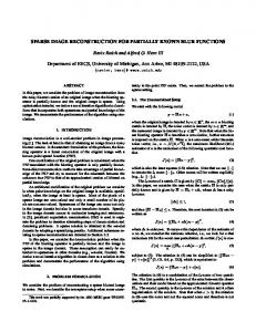
1. Radio Interferometry
(E)VLA - http ://www.aoc.nrao.edu/evla/
Example of a 4-hour sampling :
3
1. Model : an underdetermined problem • Underdetermined system :
y =
F
P
x+n
x ∈ R+N : image of interest (unknown) P : Primary beam F : Fourier transform (FFT) matrix restricted to the set of probed frequencies y ∈ CM : data points (visibilities) in Fourier spectrum at sampled frequencies n ∈ CM , n ∼ CN (0, Σ) • N > M → Infinity of solutions in general • Prior knowledge : x has few "main features" (x is close to sparse) • Sparsity : via representation bases or redundant dictionaries 4
,
2. Sparsity : Example of the DCT basis
Best non-linear approximation in DCT : snr = 17.99 dB ; in I : snr = 0.34 dB 5
2. Redundant dictionaries • Large variety of available representations, e.g., Direct space (B = I), Discrete Cosine Transform (DCT), Wavelets, Curvelets, Bandlets,... • The choice of a representation is made w.r.t. a class of signals and for images depends on the existence of fast operators • Can concatenate representations bases Bi in a dictionary of T > N vectors, then x ≈ Du with D = [B1 B2 . . . BK ], and u ∈ RT is sparse
• Resulting redundant dictionaries increase the richness of the geometrical a priori but make the approximation problem more difficult 6
2. Sparsity and approximation • A Sparse approximation of x can be obtained by a few atoms Di (vectors) of some representation dictionary D = {Di}i=1,...,T with coefficients ui :
• The model y = F P x + n becomes : y = F P Du + n
with u sparse
⇒ The reconstruction can be seen as a sparse denoising problem • The noise is not i.i.d. : n ∼ CN (0, Σ) 7
2. MAP interpretation and Sparse Priors • Model : where
y = F P D u + n, x = Du and n ∼ CN (0, Σ) .
• Maximum A Posteriori : probabilistic setting on u. MAP defined by b MAP = arg max p(y|u), with p(y|u) ∝ L(y; u)p(u) u u
log p(u)} = arg min − log L(y; u) − | {z u
|
{z D(u,y)
}
Π(u)
= arg min ||y − F P Du||2 Σ + Π(u) u
1 −1 − F P D} u||2 + Π(u). = arg min || Σ 2 y − |Σ 2{z u | {z } Dν z
• Transformed dictionary : Dν = Σ • Sparse prior : Π(u) • Model with whitened data : 1
−1 2
1
1
FPD
1
−2 −2 −2 Σ− 2 y = Σ F P D u + Σ n , with � = Σ n ∼ CN (0, I) | {z } | {z } | {z } z
Dν
�
8
2. Sparsity Inducing Reconstruction, D = Union of bases −1 • Model : z = Σ F P D} u + �, with � ∼ CN (0, I) | 2{z Dν Dν : transformed dictionary z }|
{
• Reconstruction approach : • Choose K sparsifying bases {Bi}i=1...K , set D = [B1 B2 . . . BK ] • Find a sparse ˜ u that well approximates z : - Minimize ||z − Dν u||2 greedily → sparse by construction - or solve : arg minu ||z − Dν u||2 + Π(u) → sparsity inducing functions • The reconstructed (synthesized) image is ˜ x = D˜ u 9
2. Illustration : F , P and Σ
10
2. Illustration : F , P and Σ
y = Fx PSF : F †y = F †F y
Σ
−1 2
y=Σ
−1 2
Fx
1 −2
y = F † Σ− 2 F x
PSF+Σ : F Σ
1
11
−1 2
y=Σ
−1 2
y = FPx
Σ
FPx
PSF+P : F †y = F †F P y
PSF+Σ+P : F Σ− 2 y = F †Σ− 2 F P x
1
1
3. Greedy approach : MP, normalized or not • Decreases ||z − Dν u||2 greedily. Algorithm : 1
• Initialisation : m = 0. r0 = z = Σ− 2 y. || • Best match : Find Dνm = argmaxi ||D || . νi m+1 m • Update : r = r − γ ||D ||2 Dνm, νm || • Criterion stop : Compare the new normalized correlations { } ||Dν i ||
to a threshold • Back projection : Reestimate {˜ ui
} =argminu0 ||z − ˜
i∈Λ
i
X
u0iDν i||2
˜ i∈Λ
• Particular case : CLEAN algorithm [Hoegbom 1974] • The performances of MP depend on : ||
k νl - the normalized correlations between atoms k and l : µk,l = ||D ν||.||D νk ν l || - the norms : ||Dν k ||. 12
3. Influences of {µk,l} and {||Dν k ||} • Example : false alarms on pure noise r = � : - Normalized : select
|| > τ , and v = ≈ N (0, 1) i ||Dν i || ||Dν i ||
- Not normalized : select | < r, Dν i > | > τ 0 with < r, Dν i >= ui||Dν i||
Normalized
Not normalized
Atom Norms
τ and τ 0 yield same average PF A 13
3. Influences of {µk,l} and {||Dν k ||} • Example : one component signal in noise r = β Dν 100 + � :
- Normalized : ||D ν||i = β µi,100.||Dν i|| + vi νi - Not normalized : < r, Dν i > | = βµi,100.||Dν i||.||Dν 100|| + vi||Dν i||
Normalized Not normalized • However, normalization may create numerical instabilities
µi,100 14
2. Atoms’ visibility
F †y = F †F By ⇒ "PSF" with B=DCT : F y = F †F Bu 15
3. Example of a fully visible DCT atom
16
3. Example of a fully invisible DCT atom
17
3. Example of a partially visible DCT atom
Note : I atoms are always visible (I and F are maximally incoherent) up to P , wavelets atoms are also localized
18
4. Sparsity inducing functions 1
1
F P D} u||2 + Π(u). • Solve arg minu J(u) = || Σ− 2 y − |Σ− 2{z | {z } z
Dν
• Thresholding functions are sparsity inducing by construction • There are many sparsity inducing penalisation / thresholding rules, e.g. − l0 norm : best expresses strict sparsity : hard thresholding in ⊥ denoising P − l1 norm (= i |ui|) often seen as a convex approximation to l0 : soft threshloding P − lp "norms", with 0 < p < 1 (= i |ui|p) : the lower p, the more sparse solution, but J(u) is not convex
19
b 4. Hard and Soft thresholdings : function x(y) 6 Hard thresholding T=1 Soft thresholding T=1 5
xest(y)
4
3
2
1
0
0
1
2
3 y
↑ Threshold point (yt, xt)
4
5
6
20
4. l0 and l1 denoising : Numerical example Original
Noisy
Original
noisy image: normalized error = 12.4277% 400
250
300 200
200 150
100
100
0
50 −100
0
||x−x ˆ||2 Normalised error : e = = 12.4% ||x||2 21
4. Compared denoising with lp "norms"
Best threshold l1 : 1.7σ Best threshold l0 : 3.4σ 22
Original
Noisy
Original
noisy image: normalized error = 12.4277% 400
250
300 200
200 150
100
100
0
50 −100
0 l0 noisy: normalized error = 2.1606%
l1 noisy: normalized error = 1.9301%
250
200 200
150 150
100
100
50
50
0 0
π = l0 : e = 2.1%
π = l1 : e = 1.9%
Sparsity of ˆ x : 1% for l0 and 10% for l1. The most sparse is not the best. 23
4. Thresholding functions of GG priors
24
4. Iterative Soft Thresholding Algorithm • Goal : solve the constrainted problem u ˜ = argminu||u||1 s.t. ||z − Dν u||2 ≤ � by minimizing its Lagrangian formulation L1 = ||z − Dν u||2 + L2||u||1 • For each �, there exists L making both problems equivalent • Algorithm : • Initialisation : m = 0. Choose u0 = 0. 0 † m) • Gradient step : u ˜m = u D (z − D u ˜ ˜m + 1 ν ν τ
0m m+1 • Soft thresholding : u˜i = ρL/τ (u˜i ) um||1 • Criterion stop : A fixed tolerance on ||˜ um+1 − ˜
• Back projection : Reestimate u ˜i
˜ i∈Λ
by minimizing ||y −
X
u ˜iDν i||2
˜ i∈Λ
• Many acceleration algorithms exist (e.g. FISTA,GPSR,SPARSA,GPAS) • Same normalization issues as for MP 25
5. Some results
26
2. Dictionary = [Dirac Wavelet] bases (data snr =39 dB) Original Image
MTF
Equivalent PSF
Peudo Inv Rec snr = 9.1512dB
27
(data snr =39 dB)
28
.
a)
=
b)
+
c)
3. Dictionary = [Dirac DCT] bases (data snr =43.1 dB) Original Image
MTF
Equivalent PSF
Peudo Inv Rec snr = 15.1911dB
29
(data snr =43.1 dB)
.
a)
=
b)
+
c)
→ feature separation → reconstruction and denoising
30
6. Summary • Interferometric image reconstruction treated as a denoising approach • Sparse denoising of weighted interferometric data by means of a few vectors that carry geometrical features of the images in union of bases • Illustrated effects of atoms norms correlations and denormalization • Redundant dictionaries generally improve on single representation bases : more geometrical a priori is available • l1 minimization generally improves the reconstruction w.r.t. greedy approaches. Other sparsity inducing functions may be considered • Started working on VLA data, other representations in the dictionary (curvelets, bandlets), comparing synthesis and analysis approaches, and comparing to other regularized deconvolution methods 31