Internal Report 99â06 A Comparative Evaluation of ... - CiteSeerX

Internal Report 99–06 A Comparative Evaluation of Matching and Tracking Object Features for the Purpose of Estimating Similar-View-Areas of 3-Dimensional Objects

by Gabriele Peters, Barbara Zitova, Christoph von der Malsburg

Ruhr-Universit¨ at Bochum Institut f¨ ur Neuroinformatik 44780 Bochum

IR-INI 99–06 April 1999 ISSN 0943-2752

c 1999 Institut f¨

ur Neuroinformatik, Ruhr-Universit¨ at Bochum, FRG

Abstract The viewing hemisphere of a 3-dimensional object can be partitioned into areas of similar views, termed view bubbles. We compare two different procedures of generating view bubbles. On the one hand, local object features are tracked from one view to another by utilizing the continuity of successive views while the object rotates. On the other hand, the features are matched in different views which are assumed to be independent. We had a quantitative and a qualitative criterion of comparison (the size of the view bubbles and view similarities inside the view bubbles, respectively). To compare the sizes of view bubbles for both procedures we performed statistical analyses. For the qualitative comparison we assessed the correspondences provided by both procedures. The simulations were done on natural images of two objects. Both procedures, tracking as well as matching, proved to be appropriate to generate a distribution of view similarities on the viewing hemisphere. Canonical views arise. We could not find a difference between both procedures concerning the quantitative size criterion, but tracking outperforms matching concerning the qualitative condition. Tracking provides much more precise correspondences than matching. The continuous information seems to be neccessary to build the correspondences. Accordingly, tracking is the more appropriate method for recognizing the changes of features, whereas matching is more suitable if features of the same appearance are to be found. Our results are supported by related insights from psychophysical research.

Contents 1 Subject of Investigation

1

2 Description of the System 2.1 Image Acquisition . . . . . . . . . . . . . . . . . 2.2 Preprocessing . . . . . . . . . . . . . . . . . . . . 2.2.1 Segmentation . . . . . . . . . . . . . . . . 2.2.2 Gabor Transform and Similarity Function 2.2.3 Grid Graphs . . . . . . . . . . . . . . . . 2.3 Matching Object Features . . . . . . . . . . . . . 2.4 Tracking Object Features . . . . . . . . . . . . . 2.5 Generation of View Bubbles . . . . . . . . . . . . 2.5.1 View Similarity for Matching . . . . . . . 2.5.2 View Similarity for Tracking . . . . . . .

. . . . . . . . . .

. . . . . . . . . .

. . . . . . . . . .

. . . . . . . . . .

. . . . . . . . . .

. . . . . . . . . .

. . . . . . . . . .

. . . . . . . . . .

. . . . . . . . . .

. . . . . . . . . .

. . . . . . . . . .

. . . . . . . . . .

. . . . . . . . . .

. . . . . . . . . .

. . . . . . . . . .

3 3 4 4 6 7 7 8 8 9 9

3 Methods of Comparision 10 3.1 Statistics . . . . . . . . . . . . . . . . . . . . . . . . . . . . . . . . . . . . . 10 3.2 Correspondences . . . . . . . . . . . . . . . . . . . . . . . . . . . . . . . . . 10 4 Results 11 4.1 Statistics . . . . . . . . . . . . . . . . . . . . . . . . . . . . . . . . . . . . . 11 4.2 Correspondences . . . . . . . . . . . . . . . . . . . . . . . . . . . . . . . . . 17 5 Discussion and Conclusion

27

6 Parallels to Human 3–Dimensional Object Recognition

29

A Appendix

30

I

Chapter 1

Subject of Investigation Our aim is to learn a viewpoint-invariant object representation which is capable of recognizing a moving or rotating object from a short sequence and estimating its pose. Our approach belongs to the kind of representations where an object is represented by an aspect graph (e.g., [6], [11], [12]). We want to partition the upper hemisphere of an object’s viewing sphere into view categories, i.e., aspects. For this purpose we first determine for each view of the hemisphere a surrounding area of similar views. This area is termed view bubble (see figure 1.1). Then the aspects of the object will be derived from the overlaps of the view bubbles. In this paper we describe the generation of the view bubbles. We compare two procedures of determining the similarity of two views: matching a representing graph of one view to another view, on the one hand, and tracking object features from one view to another view, on the other hand. During the matching procedure each view is treated independently, whereas the tracking procedure utilizes the continuity of neighbouring views. Our investigations were guided by the question which procedure - matching or tracking is more appropriate to find for each view of the hemisphere view bubbles of maximal size containing views of maximal similarity? We used two methods to compare both procedures. First we made statistical analyses to examine the size of the view bubbles, and second we assessed the correspondences provided by both procedures to judge the view similarities inside the view bubbles.

1

2

c 1999 Institut f¨ IR-INI 99–06, ur Neuroinformatik, Ruhr-Universit¨ at Bochum, FRG

view (79, 14)

Tom

dwarf

view (6, 6)

Tom

dwarf

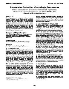
Figure 1.1: Viewing Hemisphere with Examples of View Bubbles. The representation of the viewing hemisphere consists of 100 × 25 views. Each crossing of the grid stands for one view. The dot in front marks view (0, 0). Two examples for view bubbles are depicted on the hemisphere grid. They have been determined with the tracking procedure for the object “Tom”. View (79, 14) provides a small view bubble. It includes views which cover a range of 21.6 degrees in x-direction, i.e., east-west direction, and 14.4 degrees in y-direction, i.e., north-south direction. View (6, 6) provides a larger view bubble, which covers a range of 43.2 degrees in x-direction and 28.8 degrees in y-direction. The referring views of the second object we have used, the “dwarf”, are shown next to the images of “Tom”. For details see description in the text.

Chapter 2

Description of the System 2.1

Image Acquisition

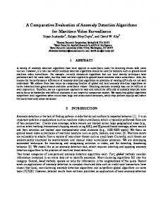
To acquire the views of the upper hemisphere of an object, we used an antropomorphic robot, which has a redundant manipulator arm with 7 degrees of freedom (DoF), kinematics similar to a human arm and a parallel jaw gripper [1]. The object was placed in the gripper of the robot, while the gripper itself was covered by a gray paper to get a homogeneous background in the images. So, the object only is visible in the images (see figure 2.1).

Figure 2.1: Robot Scene. The robot arm has object “Tom” fixed in its gripper. The gripper itself is covered by a gray background. Then the arm moved in a way that the object rotated around its center while a camera recorded the views. The arm moved in steps of 3.6 degrees in either direction, north-south and east-west direction. So, the upper viewing hemisphere of an object is covered by 2500 views: 100 views for each circle of the east-west movement and 25 views for each longitude from the “equator” to the “north pole” (see again figure 1.1). We recorded gray level images of size 128 × 128 with 256 gray levels. 3

4


2.2

Preprocessing

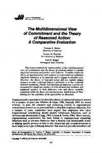
For each recorded view of an object we first perform a segmentation based on gray levels which separates the object from the background. Then we put a grid graph onto the segment of the image which has been assigned to the object. At each vertex of the graph we extract features which describe the surroundings of the vertex, i.e., local features of the special view of the object. Thus we derive a representation for each view in form of a model graph which provides the basis of both, the matching and the tracking procedure (see figure 2.2). In subsection 2.2.1 we describe the segmentation of one image, in sub-

a)

b)

c)

d)

e)

f)

Figure 2.2: Preprocessing. a) Original image, b) Result of the gray level segmentation, c) Result after eliminating wrong segments (“centered segmentation”), d) Original image masked with the result of the centered segmentation, e) Grid graph covering the object segment, f) Grid graph shown on the original image. section 2.2.2 we give an overview of the image preprocessing with Gabor wavelets, and in subsection 2.2.3 we describe how a graph which represents one view is generated from the results of the segmentation and the Gabor transform.

2.2.1

Segmentation

The segmentation method is based on the system of [14] and described in [2]. The segmentation model contains Potts spins with coarse-to-fine dynamics comparable to real-space renormalisation methods often used in theoretical physics. Average intensity is used as the only low-level cue, although the system is able to make use of additional cues if they become available. The segmentation model divides an incoming image of some fixed resolution into N small patches Ii , i = {1, 2, ..., N }. Each surface receives a label Si , i = {1, 2, ..., N } that encodes its membership of one of several possible segments (see figure 2.3 A–C). Because of the analogy between this label-based model and an interacting spin system in solid state


A

B

C

5

D

Figure 2.3: Segmentation Model. The complex scene shown in A is divided into 32 × 32 = 1024 patches in B. C shows the corresponding randomly initialized spin image for k = 3, in which each spin value is displayed as the appropriate gray level. D illustrates the renormalisation of the interaction between spins on different resolution levels (arrows on left) and the coarse-to-fine dynamics (arrows on right).

physics, we call such a label a spin. The range of values, k, allowed for a spin Si ∈ {1, 2, ..., k}, is a parameter of the system and is set to k = 2, because we want to separate only two segments, the object and the background. We use N = 32 × 32 = 1024 spins, resulting in patches of 4 × 4 = 16 pixels per spin for our images of size 128 × 128. The aim now is to find the spin configuration which encodes the “correct” segmentation of the given scene. Each spin Si interacts with all other spins Sj via an interaction matrix Wij . The difference in mean intensity Ii − Ij at the corresponding image regions is used to compute the interaction Wij between the two spins Si and Sj assigned to these positions - the desired segmentation is mapped onto the global minimum of the following energy function: E (S) = −

N N X 1X Wij · δSi ,Sj 2 i=1

with

(2.1)

j=1j6=i

Wij = max 1 − Ii − Ij /α, 0 − W

(2.2)

The parameter α – we use α = 100 – in combination with the maximum function ensures that the difference in average intensity on the interval [0, α] is mapped to [0, 1]. To stress the Gestalt law of neighborhood [15], we restrict the interaction to spins with distances below 7.1 spins. In order to map low similarity to negative interaction and high similarity to positive one, we subtract the mean interaction W from all similarity values to obtain the used interaction Wij . We use the Metropolis [9] algorithm at zero temperature with coarse-to-fine dynamics to let the system relax to a local energy minimum (see figure 2.3 D and [2] for details). We have used 3 stages and N (1) = 1024 as the number of spins in the highest resolution. The number of spins in each resolution is given by N (n) = N (1) · 2−2(n−1). The segmentation as described may also provide regions, which are regarded as belonging to the object due to their gray levels, but in fact do not belong to it, like shadows or reflections. We get rid of them by simply choosing that segment as object, which is closest to the center of the image. Figure 2.2 c) shows the result of this centered segmentation.

6


2.2.2

Gabor Transform and Similarity Function

The original image is convolved with a family of Gabor kernels ψ~k . The parameter ~k determines the wavelength and orientation of the kernel ψ~k . The kernels in image coordinates take the form of a plane wave restricted by a Gaussian envelope function: ~k 2 ~k 2~x2 ψ~k (~ x) = 2 exp − 2 σ 2σ

!

h

i

exp i~k~x − exp −σ 2 /2

.

(2.3)

The first term in the square brackets determines the oscillatory part of the kernel. The second term compensates for the dc-value of the kernel, to avoid unwanted dependence of the filter response on the absolute intensity of the image. The complex valued ψ~k combine an even (cosine-type) and odd (sine-type) part (see figure 2.4). If I(~x) is the gray

a)

b)

Figure 2.4: Shape of a Wavelet. a) The real part (cosine phase). b) The imaginary part (sine phase). All kernels have the same shape except for size and orientation.

level distribution of the input image, the operator W symbolizes the convolution with all possible ~k: Z (WI) ~k, x~0 := ψ~k (x~0 − ~x) I (~x) d2 x = ψ~k ∗ I (x~0 ) . (2.4)

Accordingly, at each image coordinate we obtain filter responses for eachGabor wavelet. Filter responses at one image coordinate x~0 form a jet J~k (x~0 ) := (WI) ~k, x~0 . For the result of the convolution is complex, we can express the ith component of a jet in terms of amplitude ai and phase φi : Ji = (ai , φi ) for i = 1, ..., n · m, if n is the number of frequencies and m is the number of directions. We chose n = 4 and m = 8.

Thus, a similarity function S˜ between two jets J and J ′ can be defined as ˜ , J ′) = S(J

X

ai a′i cos(φi − φ′i )

i

sX i

a2i

X

2 a′ i

,

(2.5)

i

which has the range [−1.0, 1.0]. To obtain the range [0.0, 1.0] we define a linearly rescaled ˜ version of S: 1 ˜ , J ′ ) + 1). (2.6) S(J , J ′ ) = · (S(J 2 S is the similarity function we used for our simulations, for the matching as well as for the tracking procedure.


2.2.3

7

Grid Graphs

Given the result from the centered segmentation we mask the original image with it. Now we can cover the whole masked image with a grid graph. We chose a grid with 13 × 13 vertices. Then all vertices are deleted, which lie on the background or which lie on the object but are too close to the background. The reason for this is to prevent vertices from incorporating too much information of the background. The minimal allowed distance to the background segment is determined by a certain fraction p of the radius of the largest Gabor kernel. We chose p = 0.1. Then each vertex is labeled with the jet, which corresponds to the position of the vertex (see figure 2.5), as described in subsection 2.2.2. For display purposes the remaining vertices are connected by a minimal spanning tree (see figure 2.2 e) and f)). Jet

Imagegraph

Figure 2.5: Jet and Graph. This jet is generated from a family of Gabor kernels with 3 frequencies and 4 directions. Each vertex of the graph is labeld with such a jet. (The graph shown in this image is not a grid graph but a free graph.)

2.3

Matching Object Features

Elastic Graph Matching is described in detail in [7]. Given a graph with vertices labeled with jets, the aim of matching this graph to an image is to find new vertex positions which optimize the similarity of the vertex labels to the features extracted at the new positions. The process of graph matching is divided into two stages. In the first stage the graph is shifted across the image while keeping its form rigid. We use steps of one pixel in either direction for this rigid shift. For each position of the graph we calculate the total similarity of the new positioned graph to the original graph. The total similarity is just the average similarity taken for each vertex by using the similarity function 2.6. This global move procedure is able to position the graph on the object. The position which provides the highest similarity is the starting position for the second stage. This second stage permits small graph distortions, i.e., the vertices are shifted locally and independently in a small surroundings of their starting position. We chose a surroundings of 5 × 5 pixels for each vertex, which was scanned in steps of one pixel in either direction. Again, the total similarity is calculated for each step. After this local move procedure the optimal position of the graph is found at the position which provides the highest total similarity (see figure 2.6).

8


grid graph

local move

global move

Figure 2.6: Matching. The grid graph which represents view (91, 4) is matched on view (96, 4). After the global move the rigid graph has found its optimal position on the object. After the local move the graph has been deformed to optimize the positions of the single vertices.

2.4

Tracking Object Features

The tracking procedure we use is described in [8] and based on [3] and [13]. Given a sequence of a moving object and the pixel position of a landmark of the object for frame n, the aim is to find the corresponding position of the landmark in frame n+1. As a visual feature we use the Gabor wavelet responses described in subsection 2.2.2. For tracking a local feature from one frame to another, a similarity function between two jets J and J ′ is defined, which differs slightly from formula 2.5:

S ′ J , J ′ , d~ :=

′

i ai ai cos

P

qP

′ φi − φi − d~~ki

2 i ai

′2 iai

P

(2.7)

with d~ being the displacement vector of the two jets and ~ki being the wave vectors of the Gabor filters. If J and J ′ are extracted at same pixel positions in the frames n and n + 1, d~ (and thus the new position of the landmark) can be found by maximizing S ′ in ~ Because the estimation of d~ is precise for small its Taylor expansion with respect to d. displacements only, i.e., large overlap of the Gabor jets, large displacement vectors are treated as a first estimate only and the process is iterated. We used four iterations. In this way displacements up to half the wavelength of the kernel with the lowest frequency can be computed (see [16] for details). For each vertex of the graph of frame n the displacements are calculated for frame n + 1. Then a graph is created with its vertices at the new corresponding positions in frame n+1, and the labels of the new vertices are extracted from the new positions. But although the displacement vectors have been determined as decimal numbers, the jets can be extracted at (natural number) pixel positions only. This would result in a systematic rounding error. To compensate for this subpixel error ∆d~ the phases of the Gabor filter responses are shifted according to ∆φi = ∆d~ · ~ki . Then they will look as if they were extracted at the correct subpixel positions (see figure 2.7).

2.5

Generation of View Bubbles

The view bubbles are areas of the viewing hemisphere, which enclose similar views of an object, as mentioned in the introduction. For each view an affiliated view bubble is


9

Figure 2.7: Tracking Local Object Features. The frames 1, 10, 20, 30, 40, and 50 of a sequence are shown here.

created, with the view as its center. To determine the view bubble for a special view, we compare neighbouring views in all directions (east, west, north, and south). If the similarities to the starting view are still sufficiently high (depending on a preset threshold, see below) we depart one step further from the starting view. In detail, if (i, j) is the view for which we want to create the bubble, we first compare views in east-west direction. We begin with the views (i − 1, j) and (i + 1, j). If both views provide a sufficiently high total similarity to the start graph we go on with the views (i − 2, j) and (i + 2, j). We stop this procedure if one of both tested views becomes too dissimilar. By doing the same for the north-south direction we obtain four views (i − n, j), (i + n, j), (i, j − m), and (i, j + m) on the hemisphere, which define the view bubble for the starting view. To depict a view bubble we draw an ellipse through these four views with the starting view as its centerr. Figure 1.1 shows two ellipses projected onto the viewing hemisphere. In the following subsections we describe the differences in the determination of the similarity between two views depending on the two procedures we want to compare, matching and tracking. For both procedures we used the same similarity threshold 0.77. (The average similarity between two randomly chosen views for one of the used objects was 0.68, determined for 15 matched views.)

2.5.1

View Similarity for Matching

For the matching procedure the grid graph, which was generated for the starting view is matched successively in the neighbouring views and the total similarity of the graph to the new view is calculated after each match as described in section 2.3.

2.5.2

View Similarity for Tracking

For the tracking procedure we start with the grid graph which was generated for the starting view. This graph is tracked to all directions. After each tracking step the same total graph similarity is computed as for the matching proedure. The difference between tracking and matching concerning the similarity of views lies in the fact that during matching the similarity is calculated always in reference to the starting view, whereas during tracking the similarity refers to the preceding view. In contrast to the matching procedure the correspondences from one view to the next are preserved during tracking.

Chapter 3

Methods of Comparision We ran our simulations with two objects, a simple one (the “dwarf”) and a more complex one (the cat “Tom”) (see figure 1.1). “Simple” means that the views of the object do not change rapidly while the object rotates. The “dwarf” is a relatively convex object with rather similar shape for all viewing directions, whereas “Tom” is a more irregular object with faster changing views. As mentioned in the introduction we used two different methods to compare the view bubbles generated by the matching (respectively tracking) procedure. With statistical analyses we made a quantitative comparison, and by judging the correspondences, which were found by both procedures, we compared matching and tracking qualitatively.

3.1

Statistics

For the quantitative comparison we had two criterions. On the one hand we determined the area of each view bubble by calculating the area of the ellipse, described in section 2.5. This condition we call area of view bubbles. On the other hand we counted for each view, in how many other view bubbles it is contained. This condition we call accumulated view bubbles. We ran simulations for both objects, both criterions and both procedures, matching and tracking. For each object and each criterion we carried out a t-test to proof the hypothesis of different means of the areas of view bubbles (respectively accumulated view bubbles) for the samples “view bubbles generated by matching” and “view bubbles generated by tracking”.

3.2

Correspondences

For the qualitative comparison we chose four sequences on the hemisphere (from a starting view to a destination view) for both objects. For each of these sequences we performed the matching and the tracking procedure. To assess the correspondences we displayed for each view of the sequences the resulting matched and tracked graphs in figures and plotted the calculated similarities in diagrams. The sequences had an average size of about 8 frames which means a covered rotation angle of 25,2 degrees. The longest sequence covers 43,2 degrees and consists of 13 frames.

10

Chapter 4

Results This chapter is divided into the section “Statistics”, where the results of the quantitative comparisons are listed, and the section “Correspondences”, where the qualitative differences between the matching and tracking procedure are described.

4.1

Statistics

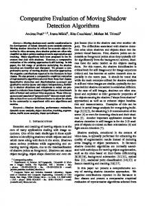
The diagrams in figures 4.1 and 4.2 show the results for the object “Tom”, figures 4.3 and 4.4 for object “dwarf”. In the figures 4.1 and 4.3 the distributions of areas of view bubbles are shown, in the figures 4.2 and 4.4 the distributions of accumulated view bubbles. For all of these four figures the first diagram depicts the results from the tracking procedure and the second diagram shows the results from the matching procedure. Light colors encode large areas (respectively large numbers of accumulated view bubbles), dark colors encode small areas of view bubbles (respectively small numbers of accumulated view bubbles). To compare the results for tracking and matching the third diagram shows the difference between the first and second diagram, i.e., the values derived from the matching procedure are subtracted from the values derived from the tracking procedure. Dark areas in the third diagram are areas of the hemisphere where tracking provides larger view bubbles (respectively larger numbers of accumulated view bubbles). From the diagrams we get following results. For both objects, “Tom” and “dwarf”, the distribution of areas of view bubbles as well as the distribution of accumulated view bubbles is qualitatively similar for the tracking procedure and for the matching procedure. The back view seen from slightly above and the front view provide the largest bubbles, and they can be regarded as canonical views. Regarding the difference between the criterions “area of view bubbles” and “accumulated view bubbles” we can say that the results look similar with the exception that the distributions for the accumulated view bubbles are smoother than for the areas of the view bubbles. These results hold for both objects, “Tom” and “dwarf”. But there is a difference between the objects. The tracking procedure provides larger view bubbles (in terms of areas of view bubbles as well as in terms of accumulated view bubbles) than the matching procedure for the majority of views for the more complex object “Tom”, whereas for the more simple object “dwarf” it is the other way around: here the matching procedure provides larger view bubbles than the tracking procedure for the majority of views. The one-tailed t-test, with which we compared the mean values, was significant with α = 1% for each case. 11

c 1999 Institut f¨ 12 IR-INI 99–06, ur Neuroinformatik, Ruhr-Universit¨ at Bochum, FRG

object TOM, TRACKED, AREA of view bubbles

y−index of view

24 19 14 9 4 9

19 mean: 33.45,

29

39

49 59 69 79 89 x−index of view standard deviation: 23.02, minimum: 0.00, maximum: 131.95

99

object TOM, MATCHED, AREA of view bubbles

y−index of view

24 19 14 9 4 9

19 mean: 29.72,

29

39


99

object TOM, Difference TRACKED − MATCHED, AREA of view bubbles

y−index of view

24 19 14 9 4 9

19

29

39

49 59 69 x−index of view light gray: = 0, white: < 0, dark gray: > 0, minimum: −37.70,

79

89

maximum: 50.27

Figure 4.1: Object “Tom”, Area of View Bubbles.

99

c 1999 Institut f¨ IR-INI 99–06, ur Neuroinformatik, Ruhr-Universit¨ at Bochum, FRG 13

object TOM, TRACKED, ACCUMULATED view bubbles

y−index of view

24 19 14 9 4 9

19

29

mean: 33.32,

39


99

object TOM, MATCHED, ACCUMULATED view bubbles

y−index of view

24 19 14 9 4 9

19 mean: 29.77,

29

39


99

object TOM, Difference TRACKED − MATCHED, ACCUMULATED view bubbles

y−index of view

24 19 14 9 4 9

19

29

39


79

89

maximum: 28.00

Figure 4.2: Object “Tom”, Accumulated View Bubbles.

99


object DWARF, TRACKED, AREA of view bubbles

y−index of view

24 19 14 9 4 9

19 mean: 41.01,

29

39


99

object DWARF, MATCHED, AREA of view bubbles

y−index of view

24 19 14 9 4 9

19 mean: 54.93,

29

39


99

object DWARF, Difference TRACKED − MATCHED, AREA of view bubbles

y−index of view

24 19 14 9 4 9

19

29

39


79

89

maximum: 47.12

Figure 4.3: Object “Dwarf”, Area of View Bubbles.

99


object DWARF, TRACKED, ACCUMULATED view bubbles

y−index of view

24 19 14 9 4 9

19 mean: 40.68,

29

39


99

object DWARF, MATCHED, ACCUMULATED view bubbles

y−index of view

24 19 14 9 4 9

19 mean: 54.29,

29

39


99

object DWARF, Difference TRACKED − MATCHED, ACCUMULATED view bubbles

y−index of view

24 19 14 9 4 9

19

29

39


79

89

maximum: 17.00

Figure 4.4: Object “Dwarf”, Accumulated View Bubbles.

99

c 1999 Institut f¨ 16 IR-INI 99–06, ur Neuroinformatik, Ruhr-Universit¨ at Bochum, FRG Some statistical values are summarized in the following tables. Tom tracking area of view bubbles

mean standard deviation minimum value maximum value

matching = = = =

t-test with α = 1.0% : accumulated view bubbles


= = = =

t-test with α = 1.0% :

33.45 23.02 0.0 131.95


T = 5.77 33.32 16.95 7.0 79.0

=⇒

=⇒

29.72 22.78 0.0 131.95

meantrack > meanmatch


T = 7.49

= = = =

= = = =

29.77 16.52 5.0 72.0

meantrack > meanmatch

Dwarf tracking area of view bubbles


matching = = = =

t-test with α = 1.0% : accumulated view bubbles


= = = =

t-test with α = 1.0% :

41.01 26.54 0.0 131.95


T = 14.16 40.68 18.82 9.0 91.0

=⇒

=⇒

54.93 41.39 0.0 263.89

meanmatch > meantrack


T = 20.26

= = = =

= = = =

54.29 27.83 9.0 138.0

meanmatch > meantrack


4.2

Correspondences

In the figures 4.5 to 4.8 some results for the sequences of the object “Tom” are shown, in the figures 4.9 to 4.12 for the object “dwarf”. In the first part of each figure we display the views of the object with the graphs resulting from the tracking procedure (first row of images) and the views of the object with the graphs resulting from the matching procedure (second row of images). Both rows start with the starting view of the sequence with its generated grid graph on the object. The next two images are chosen according to the quality of the matching. We show the view with its graph where matching provided the last successfully matched graph in the sequence. The subsequent image depicts the view with the first mismatched graph of the sequence. Arrows point to the mismatched vertices. The last images of the rows show the last views of the sequence where the tracked graph still keeps the corresponding points, whereas the matched graph does not. In the headers of the images the indices of the views can be read. “Tr” means “tracked”, “Mt” means “matched”. For these images only show a part of the whole sequences, the whole sequences with their tracked and matched graphs are depicted in the appendix A. The second part of each figure shows a diagram where the similarities for each view of the sequence to the starting view is plotted for the tracked as well as the matched graphs. The similarities decrease monotonously while the object rotates away from the starting view, for the tracking procedure as well as for matching. From the assessment of the positions of the vertices of the tracked and matched graphs we can make the statement that for each view of each sequence the tracking procedure provides the same or better correspondences than the matching procedure. For the last view of each sequence the tracking procedure provides considerably better correspondences than matching. From the similarity diagrams we get the following result. At the beginning of a sequence the tracking procedure always provides higher similarities than the matching procedure. This relationship is reversed at that point of the sequence where the matching starts to provide poor correspondences, whereas tracking provides good correspondences until the end of the sequence (see figure 4.13).


TOM, sequence (91,4) -> (99,4)

tracked:

...

...

matched:

...

... last good match

first poor match

TOM, sequence (91,4) −> (99,4) 1

0.95

similarity to image (91,4)

0.9

0.85

0.8

← first poor match

0.75

0.7

0.65 (91,4)

(92,4)

(93,4)

(94,4) (95,4) (96,4) (97,4) (x,y)−index of sequence images solid line: tracked dashed line: matched

Figure 4.5: Object “Tom”, First Sequence.

(98,4)

(99,4)


TOM, sequence (48,5) -> (36,5)

tracked:

...

...

matched:

...

... last good match

first poor match

TOM, sequence (48,5) −> (36,5) 1

0.95


0.9

0.85

0.8 ← first poor match 0.75

0.7

0.65

0.6 (48,5)

(47,5)

(46,5)

(45,5)

(44,5) (43,5) (42,5) (41,5) (40,5) (39,5) (x,y)−index of sequence images solid line: tracked dashed line: matched

Figure 4.6: Object “Tom”, Second Sequence.

(38,5)

(37,5)

(36,5)


TOM, sequence (40,6) -> (49,6)

tracked:

...

...

matched:

...

... last good match

first poor match

TOM, sequence (40,6) −> (49,6) 1


0.95

0.9

← first poor match

0.85

0.8

0.75

0.7 (40,6)

(41,6)

(42,6)

(43,6) (44,6) (45,6) (46,6) (x,y)−index of sequence images solid line: tracked dashed line: matched

(47,6)

Figure 4.7: Object “Tom”, Third Sequence.

(48,6)

(49,6)


TOM, sequence (97,4) -> (97,11)

tracked:

...

...

matched:

...

... last good match

first poor match

TOM, sequence (97,4) −> (97,11) 1

0.95


0.9

0.85 first poor match → 0.8

0.75

0.7

0.65 (97,4)

(97,5)

(97,6)

(97,7) (97,8) (97,9) (x,y)−index of sequence images solid line: tracked dashed line: matched

Figure 4.8: Object “Tom”, Fourth Sequence.

(97,10)

(97,11)


DWARF, sequence (53,18) -> (60,18)

tracked:

...

...

matched:

...

... last good match

first poor match

DWARF, sequence (53,18) −> (60,18) 1


0.95

0.9

0.85 ← first poor match 0.8

0.75

0.7 (53,18)

(54,18)

(55,18)


Figure 4.9: Object “Dwarf”, First Sequence.

(59,18)

(60,18)


DWARF, sequence (80,6) -> (80,12)

tracked:

...

...

matched:

...

... last good match

first poor match

DWARF, sequence (80,6) −> (80,12) 1


0.95

0.9

0.85 ← first poor match

0.8

0.75

0.7 (80,6)

(80,7)


Figure 4.10: Object “Dwarf”, Second Sequence.

(80,11)

(80,12)


DWARF, sequence (85,4) -> (85,10)

tracked:

...

matched:

... last good match

first poor match

DWARF, sequence (85,4) −> (85,10) 1


0.95

0.9

0.85 first poor match →

0.8

0.75 (85,4)

(85,5)


Figure 4.11: Object “Dwarf”, Third Sequence.

(85,9)

(85,10)


DWARF, sequence (64,18) -> (71,18)

tracked:

...

...

matched:

...

... last good match

first poor match

DWARF, sequence (64,18) −> (71,18) 1

0.95


0.9

0.85 ← first poor match

0.8

0.75

0.7

0.65

0.6 (64,18)

(65,18)

(66,18)


Figure 4.12: Object “Dwarf”, Fourth Sequence.

(70,18)

(71,18)

similarity


tracking matching

{ {

sequence

poor matching

{

good matching

good tracking Figure 4.13: Qualitative Similarity Diagram. “Good” and ”poor” is meant in the sense of correct, respectively incorrect, correspondences. See description in the text for details.

Chapter 5

Discussion and Conclusion We have compared two different procedures for finding similarities in neighbouring views of a 3–dimensional object. We worked on natural images, and the processing of the images operates automatically. A disadvantage of this automatical processing is that in some cases a relative poor result of the segmentation of the images leads to a representing grid graph which does not cover the whole object (as, for example, in figure 4.9) or which covers parts of the background. But as these problems occur for both compared procedures, we claim that they did not influence our results. Both procedures, matching and tracking of object features, are suitable to generate a distribution of view similarities on the viewing hemisphere of a 3–dimensional object. On the hemisphere areas of large and of small view bubbles arise. Centers of areas of large view bubbles can be regarded as canonical views (see figure 5.1).

canonical

view (47, 6)

non-canonical

view (6, 5)

view (10, 20)

view (80, 21)

Figure 5.1: Canonical and Non-Canonical Views for Object “Tom”. View (47, 6) is the view with the largest area of its view bubble (generated by the tracking procedure). Its view bubble covers an angle of 50.4 degrees in x-direction and 43.2 degrees in y-direction. View (47, 6) can be regarded as canonical view, as well as view (6, 5). The views (10, 20) and (80, 21), for example, provide very small view bubbles only. Please, compare with the first diagram of figure 4.1. The question, our investigations were guided by, was if one of the procedures, matching or tracking of object features, outperforms the other in finding areas of similar views on the viewing hemisphere. These areas (view bubbles) should meet a quantitative and a qualitative requirement, i.e., they should be of maximum size and they should contain maximum similar views. 27

c 1999 Institut f¨ 28 IR-INI 99–06, ur Neuroinformatik, Ruhr-Universit¨ at Bochum, FRG Regarding this question we detected no difference between matching and tracking concering the size of the view bubbles, but we found much more precise correspondences provided by tracking than by matching. In detail, from both test objects no statement was possible about the superiority of one procedure in terms of size of view bubbles, because for the more complex object “Tom” tracking provided larger view bubbles, whereas matching outperformed tracking for the simpler object “dwarf”. A possible explanation for this result could be that the rapidly changing views of object “Tom” cannot be matched over larger distances, because the matching procedure is looking for the same appearance of the object features, whereas the tracking procedure reacts more sensible when views are changing during the rotation of the object. A hypothesis we derived from the statistics is that the tracking procedure leads to larger view bubbles than the matching procedure for “complex” objects, whereas matching is superior to tracking for “simple” objects. But this hypothesis has to be verified for more examples. A reason for the more precise correspondences found by tracking could be the fact that an object feature changes its appearence while the object rotates. The feature in the tracking procedure adapts to this change, whereas the matching procedure always searches for the same starting feature. The more the rotation proceeds the more difficult it is for the matching procedure to find the correct point. The advantage of tracking of object features is that it “joins in” the rotation. Continuous information is used by the tracking procedure in contrast to the matching procedure. Matching is the more appropriate method if the task is to find features with the same appearance, tracking is the more appropriate method if changes of the features should be followed. Even if it would turn out that matching is superior to tracking for simple objects in terms of size of the view bubbles we consider the qualitative requirement to be more important. Precise correspondences should take priority over larger view bubbles, particularly for further processing. For a view interpolation, for example, precise correspondences are necessary, and to establish these correspondences, the continuity information of successive views has to be utilized. Accordingly, our final conclusion is that tracking of object features is superior to matching for estimating similar view areas of 3–dimensional objects, especially for complex objects.

Chapter 6

Parallels to Human 3–Dimensional Object Recognition Our data suggests that the tracking procedure provides more precise correspondences in neighbouring views of a 3–dimensional object than the matching procedure. In other words, good correspondences are derived from the continuity of successive views and not from (the same) disconnected static views. This result is supported by the psychophysical research of P. J. Kellman. His experiments with infants suggest that they have the ability to perceive the 3-dimensional form of an object only if information about continuous optical transformations given by motion is available [5]. They are not able to apprehend the overall form of an object from static views, even if they are multiple or sequential. This holds true for even eight months old infants. (Adults, however, are able to perceive 3-dimensional form from static views of objects. The recognition from static views seems to lean on extrapolations to the whole form based on simplicity or symmetry considerations, which may be products of learning, whereas the other mechanism is innate or early-developing.) T. Niemann et al. [10] report on experiments with parts of statues of human figures on a turntable. The eye movements of subjects watching the rotating objects were recorded. They found the eye movements often directed to the same details seen from different vantage points. This also supports the relevance of tracking of local features. Another argument is furnished by K. L. Harman and G. K. Humphrey [4]. They claim the generation of different 3-dimensional object representations, depending on the presentation of either regular or random sequences of views of the object. When a sequence of rotation is encoded, the associated temporal context may lead to the construction of a linked, higherorder system of representations for a given object. Whereas without temporal context, a single representation of each object rotation may be constructed.

29

Appendix A

TOM, sequence (91,4) -> (99,4)

first poor match Figure A.1: Object “Tom”, First Sequence. 30


TOM, sequence (48,5) -> (36,5) TOM, sequence (48,5) -> (36,5)

first poor match

Figure A.2: Object “Tom”, Second Sequence.


TOM, sequence (40,6) -> (49,6)

first poor match Figure A.3: Object “Tom”, Third Sequence.


TOM, sequence (97,4) -> (97,11)

first poor match

Figure A.4: Object “Tom”, Fourth Sequence.


DWARF, sequence (53,18) -> (60,18)

first poor match Figure A.5: Object “Dwarf”, First Sequence.


DWARF, sequence (80,6) -> (80,12)

first poor match

Figure A.6: Object “Dwarf”, Second Sequence.


DWARF, sequence (85,4) -> (85,10)

first poor match Figure A.7: Object “Dwarf”, Third Sequence.


DWARF, sequence (64,18) -> (71,18)

first poor match Figure A.8: Object “Dwarf”, Fourth Sequence.

Bibliography [1] M. Becker, E. Kefalea, E. Ma¨el, C. v. d. Malsburg, M. Pagel, J. Triesch, J. C. Vorbr¨ uggen, and S. Zadel. GripSee: A Robot for Visually-Guided Grasping. In Proceedings of ICANN International Conference on Artificial Neural Networks, Sk¨ ovde, Sweden, September 1998. [2] C. Eckes and J. C. Vorbr¨ uggen. Combining Data-Driven and Model-Based Cues for Segmentation of Video Sequences. In Proceedings WCNN96, pages 868–875, San Diego, CA, USA, 16–18 September, 1996. INNS Press & Lawrence Erlbaum Ass. [3] D. J. Fleet and A. D. Jepson. Computation of Component Image Velocity from Local Phase Information. International Journal of Computer Vision, 5(1):77, 1990. [4] K. L. Harman and G. K. Humphrey. Encoding ‘Regular’ and ‘Random’ Sequences of Views of Novel 3D Objects Rotating in Depth. IOVS: Investigative Ophthalmology & Visual Science, 39(4), 1998. [5] P. J. Kellman. Perception of Three-Dimensional Form in Infancy. Perception and Psychophysics, 36:353–358, 1984. [6] J. J. Koenderink and A. J. v. Doorn. The Internal Representation of Solid Shape with Respect to Vision. Biological Cybernetics, 32:211–216, 1979. [7] M. Lades, J. C. Vorbr¨ uggen, J. Buhmann, J. Lange, C. v. d. Malsburg, R. P. W¨ urtz, and W. Konen. Distortion Invariant Object Recognition in the Dynamic Link Architecture. IEEE Transactions on Computers, 42:300–311, 1993. [8] T. Maurer and C. v. d. Malsburg. Tracking and Learning Graphs and Pose on Image Sequences of Faces. In Proceedings of the 2nd International Conference on Automatic Face- and Gesture- Recognition, pages 176–181, Killington, Vermont, USA, October 1996. [9] N. Metropolis, A. Rosenbluth, M. Rosenbluth, A. Teller, and E. Teller. Introduction of the Metropolis Algorithm for Molecular-Dynamics Simulation. J. Chem. Phys., 21:1987, 1953. [10] T. Niemann, M. Lappe, and K.-P. Hoffmann. Visual Inspection of Three-Dimensional Objects by Human Observers. Perception, 25:1027–1042, 1996. [11] H. W. Plantinga and C. R. Dyer. Visibility, Occlusion, and the Aspect Graph. International Journal of Computer Vision, 5(2):137–160, 1990. 38

c 1999 Institut f¨ IR-INI 99–06, ur Neuroinformatik, Ruhr-Universit¨ at Bochum, FRG 39 [12] M. Seibert and A. M. Waxman. Adaptive 3-D Object Recognition from Multiple Views. IEEE Transactions on Pattern Analysis and Machine Intelligence, 14(2):107– 124, 1992. [13] W. M. Theimer and H. A. Mallot. Phase-Based Binocular Vergence Control and Depth Reconstruction using Active Vision. CVGIP: Image Understanding, 60(3):343, 1994. [14] Jan C. Vorbr¨ uggen. Zwei Modelle zur datengetriebenen Segmentierung visueller Daten, volume 47 of Reihe Physik. Verlag Harri Deutsch, Thun, Frankfurt am Main, 1995. [15] M. Wertheimer. Untersuchung zur Lehre von der Gestalt II. Forschung, 4:301–350, 1923.

Psychologische

[16] L. Wiskott. Labeled Graphs and Dynamic Link Matching for Face Recognition and Scene Analysis, volume 53 of Reihe Physik. Verlag Harri Deutsch, Thun, Frankfurt am Main, 1995.

Acknowledgement We like to thank Michael Neef for system administration, Uta Schwalm for office administration, and Pervez Mirza for proof-reading.

Internal Report 99â06 A Comparative Evaluation of ... - CiteSeerX

Internal Report 99â06 A Comparative Evaluation of ... - CiteSeerX

Suggest Documents

Internal Report - CiteSeerX

VTD Internal Report - CiteSeerX

A Comparative Performance Evaluation of DCCP - CiteSeerX

A Comparative Performance Evaluation of DCCP - CiteSeerX

A Comparative Performance Evaluation of DCCP - CiteSeerX

A Comparative Evaluation of Personality Estimation ... - CiteSeerX

A Comparative Performance Evaluation of DCCP - CiteSeerX

A comparative performance evaluation of different ... - CiteSeerX

A Comparative Evaluation of Anomaly Detection ... - CiteSeerX

COMPARATIVE EVALUATION Of CENTRALIZED ... - CiteSeerX

California Institute of Technology Internal Report ... - CiteSeerX

Comparative Recommender System Evaluation - CiteSeerX

A Comparative Evaluation of a New Unsupervised ... - CiteSeerX

Disseminating a Model for Internal Evaluation of ... - CiteSeerX

A Comparative Evaluation

Custom Test Report: Comparative Performance Evaluation

Comparative Evaluation of Moving Shadow Detection ... - CiteSeerX

Comparative Evaluation of Latency Reducing and ... - CiteSeerX

Comparative Evaluation of JavaScript Frameworks - CiteSeerX

Comparative Evaluation of JavaScript Frameworks - CiteSeerX

Comparative Evaluation of Microarray-based Gene ... - CiteSeerX

Comparative Evaluation of Environmental Flow ... - CiteSeerX

Comparative Evaluation of Robotic Software Integration ... - CiteSeerX

Comparative Evaluation of Various MFCC ... - CiteSeerX

Internal Report 99â06 A Comparative Evaluation of ... - CiteSeerX