Oct 20, 2010 ... Keywords: simulation, algorithms, spiking neural networks, ... scientists prefer to
rely on their own simulation code, often written in Matlab. ... (for example, in
NMODL for Neuron (Hines and Carnevale, 2000), or in C for NEST).
Vectorised algorithms for spiking neural network simulation Romain Brette1,2 and Dan F. M. Goodman1,2 1
Laboratoire Psychologie de la Perception, CNRS and Universit´ e Paris Descartes, Paris, France 2
D´ epartement d’Etudes Cognitives, Ecole Normale Sup´ erieure, Paris, France
October 20, 2010 Abstract High-level languages (Matlab, Python) are popular in neuroscience because they are flexible and accelerate development. However, for simulating spiking neural networks, the cost of interpretation is a bottleneck. We describe a set of algorithms to simulate large spiking neural networks efficiently with high-level languages using vector-based operations. These algorithms constitute the core of Brian, a spiking neural network simulator written in the Python language. Vectorised simulation makes it possible to combine the flexibility of high-level languages with the computational efficiency usually associated with compiled languages.
Keywords: simulation, algorithms, spiking neural networks, integrate-and-fire, vectorisation
1
Introduction
Computational modelling has become a popular approach to understand the nervous system and link experimental findings at different scales, from ion channels to behaviour. Although there are several mature neural network simulators (Brette et al., 2007), which can simulate complex biophysical models, including Neuron (Carnevale and Hines, 2006) and Genesis (Bower and Beeman, 1998), or very large-scale spiking models, for example NEST (Gewaltig and Diesmann, 2007), many scientists prefer to rely on their own simulation code, often written in Matlab. One reason might be that custom code allows more flexible development and control over the models, while in compiled simulators, using a non-standard model involves writing an extension, which is not straightforward (for example, in NMODL for Neuron (Hines and Carnevale, 2000), or in C for NEST). However, implementing simulations using hand-written code rather than dedicated simulation software has several disadvantages. First of all, code written by individual scientists is more likely to contain bugs than simulators which have been intensively worked on and tested. This may lead to difficulties in reproducing the results of such simulations (Djurfeldt et al., 2007; Schutter, 2008; Cannon et al., 2007). In addition, hand-written code can be more difficult to understand, which may slow the rate of scientific progress. Several initiatives are underway to develop standardised markup languages for simulations in computational neuroscience (Goddard et al., 2001; Garny et al., 2008; Morse, 2007), in order to address issues of reproducibility. However, these do not address the issue of flexibility, which has driven many scientists to write their own code. To address this issue, we developed a simulator written in Python (Goodman and Brette, 2009), which is a high-level interpreted language with dynamic typing. This allows the user to define their own custom model in the script and easily interact with the simulation, while benefiting from a variety of libraries for scientific computing and visualisation that are freely available. All of the major simulation packages now include Python interfaces (Eppler et al., 2008; Hines et al., 2009) and the PyNN project (Davison et al., 2008) is working towards providing a unified interface to them, but these are only interfaces to the compiled code of the simulators, and therefore do not solve the flexibility problem. In the Brian simulator, the core of simulations is written in Python. This allows the user to easily define new models, but the obvious problem with this choice is that programs usually run much slower with an interpreted language than with a compiled language. To address this problem, we developed vectorisation algorithms which minimize the number of interpreted operations, so that the performance approaches that of compiled simulators.
1
Vectorising code is the strategy of minimising the amount of time spent in interpreted code compared to highly optimised array functions, which operate on a large number of values in a single operation. For example, the loop for i in range(0,N): z[i]=x[i]+y[i] can be vectorised as z =x+y, where x, y and z are vectors of length N . In the original code, the number of interpreted operations is proportional to N . In the vectorised code, there are only two interpreted operations and two vectorised ones. Thus, if N is large, interpretation takes a negligible amount of time, compared to compiled vector-based operations. In Python with the Numpy scientific package, the operation above is about 40 times faster when it is vectorised for N = 1000. In clock-driven simulations, all neurons are synchronously updated at every tick of the clock. If all models have the same functional form (but possibly different parameter values), then the same operations are executed many times with different values. Thus, these operations can be easily vectorised and if the network contains many neurons, then the interpretation overhead becomes negligible. Neuron models can usually be described as differential equations and discrete events (spikes), so that the simulation time can be divided into the cost of updating neuron states and of propagating spikes, summarised in the following formula (Brette et al., 2007): Update N cU × dt
+ Propagation + cP × F × N × p
where cU is the cost of one update and cP is the cost of one spike propagation, N is the number of neurons, p is the number of synapses per neuron, F is the average firing rate and dt is the time step (the cost is for one second of biological time). The principle of vectorisation is to balance each interpreted operation with a vector-based operation that acts on many values, so that the proportion of time spent in interpretation vanishes as the number of neurons or synapses increases. In general, this amounts to replacing all loops by vector-based operations, but this is not a systematic rule: a loop can be kept if each operation inside the loop is vectorised. For example, if update is vectorised over neurons and propagation is vectorised over synapses (i.e., the action of one outgoing spike on all target neurons is executed in one vector-based operation), then the simulation cost is: Update + cU × N + cI + dt
Propagation F × N × (cP × p + cI )
where cI is the interpretation cost. If both N and p are large, then interpretation does not degrade simulation speed. We will start by presenting data structures that are appropriate for vectorised algorithms (section 2). We will then show how to build a network in a vectorised way (section 3), before presenting our vectorised algorithms for neural simulation (section 4). These include state updates, threshold and reset, spike propagation, delays and synaptic plasticity (section 5). Similar data structures and algorithms were already used in previous simulators (Brette et al., 2007), but not in the context of vectorisation. In this paper, we will illustrate the structures and algorithms with code written in Python using the Numpy library for vector-based operations, but most algorithms can also be adapted to Matlab or Scilab. The algorithms are implemented in the Brian simulator, which can be downloaded from http://briansimulator.org. It is open source and freely available under the CeCILL license (compatible with the GPL license). Appendix B shows the Python code for a complete example simulation, which is independent of the Brian simulator.
2 2.1
Models and data structures Vectorised containers
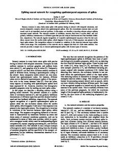
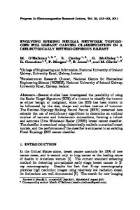
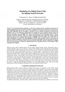
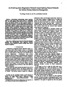
We use several combinations of some basic data structures designed for easy vectorisation. These structures are illustrated in Figure 1.
2
A
Dynamic array
B
C
Circular array
Cylindrical array Insert
Insert Insert Insert Insert
Figure 1: Basic structures. A dynamic array is an array with unused space (grey squares), which is resized by a fixed factor (here, 2) when it is full. A circular array is implemented as an array with a cursor indicating the current position. A cylindrical array is implemented as a two-dimensional array with a cursor indicating the current position. Insertion can be easily vectorised. 2.1.1
Dynamic arrays
A dynamic array is a standard data structure (used, for example, in most implementations of the C++ STL vector class, and for Python’s list class) that allows for both fast indexing and resizing. It is a linear array with some possibly unused space at the end. When we want to append a new element to the dynamic array, if there is unused space we place the element there, otherwise we resize the array to make space for the new elements. In detail, it is an array val of length n in which the first m ≤ n elements are used and the remainder are free. When an element is appended to the dynamic array, if m < n then the new element is simply placed in val[m] and m is increased by 1. If m = n (the array is full), then the array is first resized to an array of length αn (for some constant α > 1) at cost O(n). Thus, every time the array is resized, the operation costs O(n) and leaves space for (α − 1)n elements. Therefore the average cost per extra element is O(n/(α − 1)n) = O(1) (this is sometimes referred to as the amortized cost per element). 2.1.2
Circular arrays
A circular array x is an array which wraps around at the end, and which can be rotated at essentially no cost. It is implemented as an array y of size N and a cursor variable indicating the current origin of the array. Indexing x is circular in the sense that x [i+N]=x[i]=y[(i+cursor)%N], where % is the modulus operator, giving the remainder after division. Rotating the array corresponds to simply changing the cursor variable. Circular arrays are convenient for storing data that only needs to be kept for a limited amount of time. New data is inserted at the origin, and the array is then rotated. After several such insertions, the data will be rotated back to the origin and overwritten by new data. The benefits of this type of array for vectorisation are that insertion and indexing are inexpensive, and it does not involve frequent allocations and deallocations of memory (which would cause memory fragmentation and cache misses as data locality would be lost). 2.1.3
Cylindrical arrays
A cylindrical array X is a two-dimensional version of a circular array. It has the property that X [t+M, i] = X[t, i] where i is a non-circular index (typically a neuron index in our case), t is a circular index (typically representing time), and M is the size of the circular dimension. In the same way as for circular arrays, it is implemented as a 2D array Y with a cursor for the first index, where the cursor points to the origin. Cylindrical arrays are then essentially circular arrays in which an array can be stored instead of a single value. The most important property of cylindrical arrays for vectorisation is that multiple elements of data can be stored at different indices in a vectorised way. For example, if we have an array V of values, and we want to store each element of V in a different position in the circular array, this can be done in a vectorised way as follows. To perform n assignments X [t_k, i_k]=v_k (k ∈ {1, . . . , n}), we can execute a single vectorised operation: X [T, I]=V, where T =(t1 , . . . , tn ), I =(i1 , . . . , in ) and V =(v1 , . . . , vn ) are three vectors. For the underlying array, it means Y [(T+cursor)%M, I]=V. 3
2.2
The state matrix
Neuron models can generally be expressed as differential equations and discrete events (Protopapas et al. 1998; Brette et al. 2007; Goodman and Brette 2008; and for a recent review of the history of the idea, Plesser and Diesmann 2009): dX = f (X) dt X ← gi (X)
upon spike from synapse i
where X is a vector describing the state of the neuron (e.g. membrane potential, excitatory and inhibitory conductance. . . ). This formulation encompasses integrate-and-fire models but also multicompartmental models with synaptic dynamics. Spikes are emitted when some threshold condition is satisfied: X ∈ A, for instance Vm ≥ θ for integrate-and-fire models or dVm /dt ≥ θ for Hodgkin-Huxley type models (where Vm = X0 , the first coordinate of X). Spikes are propagated to target neurons, possibly with a transmission delay, where they modify the value of a state variable (X ← gi (X)). For integrate-and-fire models, the membrane potential is reset when a spike is produced: X ← r(X). Some models are expressed in an integrated form, as a linear superposition of postsynaptic potentials (PSPs), for example the spike response model (Gerstner and Kistler, 2002): X X wi V (t) = P SP (t − ti ) + Vrest i
ti
where V (t) is the membrane potential, Vrest is the rest potential, wi is the synaptic weight of synapse i, and ti are the timings of the spikes coming from synapse i. This model can be rewritten as a hybrid system, by expressing the PSP as the solution of a linear differential system. For example, consider an α-function: P SP (t) = (t/τ )e1−t/τ . This PSP is the integrated formulation of the associated kinetic model: τ g˙ = y − g, τ y˙ = −y, where presynaptic spikes act on y (that is, cause an instantaneous increase in y), so that the model can be reformulated as follows: dV dt dg τ dt g
τ
=
Vrest − V + g
=
−g
← g + wi
upon spike from synapse i
Virtually all post-synaptic potentials or currents described in the literature (e.g. bi-exponential functions) can be expressed this way. Several authors have described the transformation from phenomenological expressions to the hybrid system formalism for synaptic conductances and currents (Destexhe et al., 1994b,a; Rotter and Diesmann, 1999; Giugliano, 2000), short-term synaptic depression (Tsodyks and Markram, 1997; Giugliano et al., 1999), and spike-timing-dependent plasticity (Song et al., 2000) (see also section 5). A systematic method to derive the equivalent differential system for a PSP (or postsynaptic current or conductance) is to use the Laplace transform or the Z-transform (K¨ ohn and W¨ org¨ otter, 1998) (see also Sanchez-Montanez 2001), by seeing the PSP as the impulse response of a linear time-invariant system (which can be seen as a filter (Jahnke et al., 1999)). It follows from the hybrid system formulation that the state of a neuron can be stored in a vector X. In general, the dimension of this vector is at least the number of synapses. However, in many models used in the literature, synapses of the same type share the same linear dynamics, so that they can be reduced to a single set of differential equations per synapse type, where all spikes coming from synapses of the same type act on the same variable (Lytton, 1996; Song et al., 2000; Morrison et al., 2005; Brette et al., 2007), as in the previous example. In this case, which we will focus on, the dimension of the state vector does not depend on the number of synapses but only on the number of synapse types, which is assumed to be small (e.g. excitatory and inhibitory). Consider a group of N neurons with the same m state variables and the same dynamics (the same differential equations). Then updating the states of these neurons involves repeating the same operations N times, which can be vectorised. We will then define a state matrix S for this group made of p rows of length N , each row defining the values of the same state variable for all N neurons. We choose this matrix orientation (rather than N rows of length p) because the vector describing one state variable for 4
the whole group is stored as a contiguous array in memory, which is more efficient for vector-based operations. It is still possible to have heterogeneous groups in this way, if parameter values (the membrane time constant for example) are different between neurons. In this case, parameters can be treated as state variables and included in the state matrix. The state of all neurons in a model is then defined by a set of state matrices, one for each neuron type, where the type is defined by the set of differential equations, threshold conditions and resets. Each state matrix has a small number of rows (the number of state variables) and a large number of columns (the number of neurons). Optimal efficiency is achieved with the smallest number of state matrices. Thus, neurons should be gathered in groups according to their models rather than functionally (e.g. layers).
2.3
Connectivity structures
2.3.1
Structures for network construction and spike propagation
When a neuron spikes, the states of all target neurons are modified (possibly after a delay), usually by adding a number to one state variable (the synaptic weight). Thus, the connectivity structure must store, for each neuron, the list of target neurons, synaptic weights and possibly transmission delays. Other variables could be stored, such as transmission probability, but these would involve the same sort of structures. Suppose we want to describe the connectivity of two groups of neurons P and Q (possibly identical or overlapping), where neurons from P project to neurons in Q. Because the structure should be appropriate for vectorised operations, we assume that each group is homogeneous (same model, but possibly different parameters) and presynaptic spikes from P all act on the same state variable in all neurons in Q. These groups could belong to larger groups. When a spike is emitted, the program needs to retrieve the list of target neurons and their corresponding synaptic weights. This is most efficient if these lists are stored as contiguous vectors in memory.
A
B
Dense 0 2 0 0
3 4 0 5
8 0 0 0
0 0 0 0
0 0 0 0
1 0 0 1
C
LIL Values Row 0 3 8 1 Row 1 2 4 Row 2 Row 3 5 1
CSR
Columns 1 2 5 0 1
Row val col
0 1 2 3 3 8 1 2 4 5 1 1 2 5 0 1 1 5
1 5
rowptr 0 3 5 5 7
D
CSRC colptr 0 1 4 5 7 row 1 0 1 3 0 0 3 index 3 0 4 5 1 2 6 Column 0 1 2 3 Row val col
0 1 2 3 3 8 1 2 4 5 1 1 2 5 0 1 1 5
rowptr 0 3 5 5 7
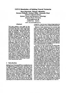
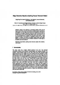
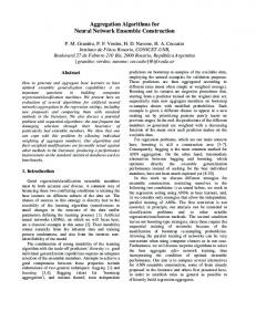
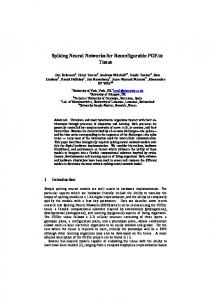
Figure 2: Matrix structures for synaptic connectivity. In all matrices, the number of rows is the size of the presynaptic neuron group and the number of columns is the size of the postsynaptic neuron group. In dense matrices, all synaptic weights are explicitly stored, where zero values signal absent or silent synapses. In the list of lists (LIL) format, only non-zero elements are stored (i.e., it is a sparse format). It consists of a list of rows, where each row is a list of column indices of non-zero elements (target neurons) and a list of their corresponding values (synaptic weights). The compressed sparse row (CSR) format is a similar sparse matrix format, but the list of rows are concatenated into two arrays containing all values (val) and all column indices (col). The position of each row in these arrays is indicated in an array rowptr. The compressed sparse row and column (CSRC) format extends the CSR format for direct column access. The array row is the transposed version of col: it indicates the row indices of non-zero elements for each column. The array index contains the position of each non-zero element in the val array, for each column. The simplest case is when these groups are densely connected together. Synaptic weights can then be stored in a (dense) matrix W, where Wi,j is the synaptic weight between neuron i in P and neuron j in Q. Here we are assuming that a given neuron does not make multiple synaptic contacts with the same postsynaptic neuron — if it does, several matrices could be used. Thus, the synaptic
5
weights for all target neurons of a neuron in P are stored as a row of W, which is contiguous in memory. Delays can be stored in a similar matrix. If connectivity is sparse, then a dense matrix is not efficient. Instead, a sparse matrix should be used (Figure 2). Because we need to retrieve rows when spikes are produced, the appropriate format is a list of rows, where each row is defined by two vectors: one defining the list of target neurons (as indices in Q) and one defining the list of synaptic weights for these neurons. When constructing the network, these are best implemented as chained lists (list of lists or LIL format), so that one can easily insert new synapses. But for spike propagation, it is more efficient to implement this structure with fixed arrays, following the CSR format (Compressed Sparse Row). The standard CSR matrix consists of three arrays val, col and rowptr. The non-zero values of the matrix are stored in the array val row by row, that is, starting with all nonzero values in row 0, then in row 1, and so on. This array has length nnz, the number of nonzero elements in the matrix. The array col has the same structure, but contains the column indices of all non-zero values, that is, the indices of the postsynaptic neurons. Finally, the array rowptr contains the position for each row in the arrays val and col, so that row i is stored in val[j] at indices j with rowptr[i] ≤ j < rowptr[i+1]. The memory requirement for this structure, assuming values are stored as 64 bit floats and indices are stored as 32 bit integers, is 12nnz bytes. This compressed format can be converted from the list format just before running the simulation (this takes about the same time as construction for 10 synapses per neuron, and much less for denser networks). As for the neuron groups, there should be as few connection matrices as possible to minimise the number of interpreted operations. Thus, synapses should be gathered according to synapse type (which state variable is modified) and neuron type (pre- and postsynaptic neuron groups) rather than functionally. Connectivity between subgroups of the same type (layers for example) should be defined using submatrices (with array views). 2.3.2
Structures for spike-timing-dependent plasticity
In models of spike-timing-dependent plasticity (STDP), both presynaptic spikes and postsynaptic spikes act on synaptic variables. In particular, when a postsynaptic spike is produced, the synaptic weights of all presynaptic neurons are modified, which means that a column of the connection matrix must be accessed, both for reading and writing. This is straightforward if this matrix is dense, but more difficult if it is sparse and stored as a list of rows. For fast column access, we augment the standard CSR matrix described above with column information to form what we will call a compressed sparse row and column (CSRC) matrix (Figure 2). We add three additional arrays index, row and colptr to the CSR matrix. These play essentially the same roles as val, col and rowptr, except that (a) they are column oriented rather than row oriented, as in a compressed sparse column (CSC) matrix, and (b) instead of storing values in val, we store the indices of the corresponding values in index. So column j consists of all elements with row indices row[i] for colptr[j] ≤ i < colptr[j+1] and values val[index[i]]. This allows us to perform vectorised operations on columns in the same way as on rows. However, the memory requirements are now 20nnz bytes, and column access will be slower than row access because of the indirection through the index array, and because the data layout is not contiguous (which will reduce cache efficiency). The memory requirements could be reduced to as low as 10nnz bytes by using 32 bit floats and 16 bit indices (as long as the number of rows and columns were both less than 216 = 65536).
2.4
Structures for storing spike times
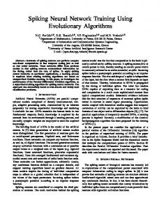
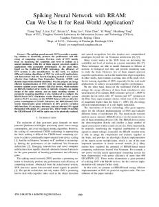
In order to implement delays and refractoriness, we need to have a structure to store the indices of neurons which have spiked recently (Figure 3). In order to minimise memory usage, this structure should only retain these indices for a fixed period (the maximum delay or refractory period). The standard structure for this sort of behavior is a circular array (see 2.1.2), which has been previously used for this purpose in non-vectorised simulations (Morrison et al., 2005; Izhikevich, 2006). Each time step, we insert the indices of all neurons that spiked in the group: x [0:len(spikes)]=spikes, and shift the cursor by len(spikes). After insertion the most recent spikes are always in x [i] for negative i . To extract the spikes produced at a given timestep in the past, we need to store a list of the locations of the spikes stored at these timesteps in the underlying array y . This is also 6
implemented in a circular array, of length duration where duration is the number of timesteps we want to remember spikes for. With this array we can insert new spikes and extract the set of indices of neurons that spiked at any given time (within duration) at a cost of only O(n) where n is the number of spikes returned. The algorithm is vectorised over spikes. The length of the circular array x depends a priori on the number of spikes produced, which is unknown before the simulation. Thus we use a dynamic array (see 2.1.1) to resize the spike container if necessary. As in the case of the standard dynamic array, this makes insertion an amortized O(1) operation. The Python code for this structure is shown in Appendix A. cursor 0 ms
2 ms
1 ms 1
2
2
3 ms
?
Unused
?
0 26
?
9
8
13
0 1 5 ms 6 ms
3
? ?
2
13 15 20 5
7 3
22 21
5
1 4
14 ms
2
22
10
5
?
25 22
4
7
4 ms
3
4
4
0
2
5
13 ms
0 1 10 ms
8 7
9
12 ms 11 ms
9 ms
8 ms
7 ms
Figure 3: Spike container. A circular dynamic array x (outer ring) stores the indices of all neurons that spiked in previous time steps, where the cursor indicates the current time step. Another circular array (inner ring) stores the location of previous time steps in the dynamic array.
3
Construction
Building and initialising the network can be time consuming. In the introduction, we presented a formula for the computational cost of a neural simulation. This expression can be mirrored for network construction by calculating the cost of initialising N neurons and constructing connection matrices with N p entries: Neurons + Connections cN × N
+ cC × N × p
where cN is the cost of initialising one neuron and cC is the cost of initialising one synapse. The cost of the second term can be quite significant, because it is comparable to the cost of simulating spike propagation for a duration 1/F , where F is the average firing rate. Vectorising neuron initialisation is straightforward, because the values of a variable for all neurons is represented by a row of the state matrix. For example, the following Python instruction initialises the second state variable of all neurons to a random value between −70 and −55: S [1,:]=-70+rand(N)*15. Vectorising the construction of connection matrices is more complex. A simple option is to vectorise over synapses. As an example, the following Brian instruction connects all pairs of neurons from the same group P with a distance-dependent weight (the topology is a ring): C.connect_full(P, P, weight=lambda i, j:cos((2*pi/N)*(i-j))) where C is the connection object, which contains the dense connection matrix C .W. When this method is called, the matrix is built row by row by calling the weight function with arguments i and j (in Python, the lambda keyword defines a function), where i is the row index and j is the vector of indices of target neurons. This is equivalent to the following Python code (using the Numpy package for vector-based operations): 7
j = arange(N) for i in range(N): C.W[i, :] = cos((2*pi/N)*(i-j)) These instructions now involve only O(N ) interpreted operations. More generally, by vectorising over synapses, the analysis of the computation cost including interpretation reads: Neurons + Connections cN × N + cI
+ N (cC × p + cI )
where cI is the interpretation cost, and the interpretation overhead is negligible when both N and p are large. With sparse matrices, both the synaptic weights and the list of target neurons must be initialised. A typical case is that of random connectivity, where any given pair of neurons has a fixed probability x of being connected and synaptic weights are constant. Again, the connection matrix can be initialised row by row as follows. Suppose the presynaptic group has N neurons and the postsynaptic group has M neurons. For each row of the connection matrix (i.e., each presynaptic neuron), pick the number k of target neurons at random according to a binomial distribution with parameters N and x. Then pick k indices at random between 0 and M − 1. These indices are the list of target neurons, and the list of synaptic weights is a constant vector of length k. With this algorithm, constructing each row involves a constant number of vector-based operations. In Python, the algorithm reads: W_target = [] W_weight = [] for i in range(N): k = binomial(M, x, 1)[0] target = sample(xrange(M), k) target.sort() W_target.append(target) W_weight.append([w]*k) where [w]*k is a list of k elements [w, w ,..., w]. Clearly, synaptic weights need not be constant and their construction can also be vectorised as previously shown.
4
Simulation
Simulating a network for one timestep consists in the following: 1) updating the state variables, 2) checking threshold conditions and resetting neurons, 3) propagating spikes. This process is illustrated in Figure 4. We now describe vectorisation algorithms for each of these steps, leaving synaptic plasticity to the next section (section 5).
4.1
State updates
Between spikes, neuron states evolve continuously according to a set of differential equations. Updating the states consists in calculating the value of the state matrix at the next time step S(t + dt), given the current value S(t). Vectorising these operations is straightforward, as we show in the next paragraphs. Figure 5 shows that with these vectorised algorithms, the interpretation time indeed vanishes for large neuron groups. 4.1.1
Linear equations
A special case is when the differential system is linear. In this case, the state vector of a neuron at time t + dt depends linearly on its state vector at time t. Therefore the following equality holds: X(t + dt) = AX(t) + B, where A and B are determined by the differential system and can be calculated at the start of the simulation (Hirsch and Smale, 1974; Rotter and Diesmann, 1999; Morrison et al., 2007). 8
A. State update
B. Threshold
C. Spike propagation
+ =
D. Reset
E. Refractoriness
Figure 4: Simulation loop. For each neuron group, the state matrix is updated according to the model differential equations. The threshold condition is tested, which gives a list of neurons that spiked in this time step. Spikes are then propagated, using the connection matrix (pink). For all spiking neurons, the weights of all target synapses (one row vector per presynaptic neuron, pink rows) are added to the row of the target state matrix that corresponds to the modified state variable (green row). Neurons that just spiked are then reset, along with neurons that spiked in previous time steps, within the refractory period. Each state vector is a column of the state matrix S. It follows that the update operation for all neurons in the group can be compactly written as a matrix product: S(t + dt) = AS(t) + BJT , where J is a vector of ones (with N elements). 4.1.2
Nonlinear equations
When equations are not linear, numerical integration schemes must be used, such as Euler or Runge-Kutta. Although these updates cannot be written as a matrix product, vectorisation is straightforward: it only requires us to substitute state vectors (rows of matrix S) to state variables in the update scheme. For example, the Euler update x(t + dt) = x(t) + f (x(t))dt is replaced by X(t + dt) = X(t) + f (X(t))dt, where the function f now acts element-wise on the vector X. 4.1.3
Stochastic equations
Stochastic differential equations can be vectorised similarly, by substituting vectors of random values to random values in the stochastic update scheme. For example, a stochastic Euler update would √ read: X(t + dt) = X(t) + f (X(t))dt + σN(t) dt, where N(t) is a vector of normally distributed random numbers. There is no specific difficulty in vectorising stochastic integration methods.
9
A
B
Figure 5: Interpretation time for state updates. A. Simulation time vs. number of neurons for vectorised state updates, with linear update and Euler integration (log scale). B. Proportion of time spent in interpretation vs. number of neurons for the same operations. Interpretation time was calculated as the simulation time with no neurons.
4.2 4.2.1
Threshold, reset and refractoriness Threshold
Spikes are produced when a threshold condition is met, defined on the state variables: X ∈ A. A typical condition would be X0 ≥ θ for an integrate-and-fire model (where Vm = X0 ), or X0 ≥ X1 for a model with adaptive threshold (where X1 is the threshold variable) (Deneve, 2008; Platkiewicz and Brette, 2010). Vectorising this operation is straightforward: 1) apply a boolean vector operation on the corresponding rows of the state matrix, e.g. S [0, :]>theta or S [0, :]>S[1, :], 2) transform the boolean vector into an array of indices of true elements, which is also a generic vector-based operation. This would be typically written as spikes=find(S[0, :]>theta), which outputs the list of all neurons that must spike in this timestep. 4.2.2
Reset
In the same way as the threshold operation, the reset consists of a number of operations on the state variables (X ← r(X)), for all neurons that spiked in the timestep. This implies: 1) selecting a submatrix of the state matrix where columns are selected according to the spikes vector (indices of spiking neurons), and 2) applying the reset operations on rows of this submatrix. For example, the vectorised code for a standard integrate-and-fire model would read: S [0, spikes]=Vr, where Vr is the reset value. For an adaptive threshold model, the threshold would additionally increase by a fixed amount: S [1, spikes]+=a. 4.2.3
Refractoriness
Absolute refractoriness in spiking neuron models generally consists in clamping the membrane potential at a reset value Vr for a predefined duration. To implement this mechanism, we need to extract the indices of all neurons that have spiked in the last k timesteps. These indices are stored contiguously in the circular array defined in section 2.4. To extract this subvector refneurons, we only need to obtain the starting index in the circular array where the spikes produced in the k th previous timestep were stored. Resetting then amounts to executing the following vectorised code:
10
S [0, refneurons]=Vr. This implicitly assumes that all neurons have the same refractory period. For heterogeneous refractoriness, we can store an array refractime of length the number of neurons, which gives the next time at which the neuron will stop being refractory. If the refractory periods are given as an array refrac, and at time t neurons with indices in the array spikes fire, we update refractime[spikes]=t+refrac[spikes]. At any time, the indices of the refractory neurons are given by the boolean array refneurons=refractime>t. Heterogeneous refractory times are more computationally expensive than homogeneous ones because the latter operation requires N comparisons (for N the number of neurons), rather than just picking out directly the indices of the neurons that have spiked (on average N × F × dt indices, where F is the average firing rate). A mixed solution that is often very efficient in practice (although no better in the worst case) is to test the condition refneurons=refractime>t only for those neurons that fired within the most recent period max(refrac) (which may include repeated indices). If the array of these indices is called candidates, then the code reads: refneurons=candidates[refractime[candidates]>t]. The mixed solution can be chosen when the size of the array candidates is smaller than the number of neurons (which is not always true if neurons can fire several times within the maximum refractory period).
4.3
Propagation of spikes A
B
Number of target neurons
Figure 6: Interpretation time for spike propagation. We measured the computation time to propagate one spike to a variable number of target neurons, using vector-based operations. A. Simulation time vs. number of target neurons per spike for spike propagation, calculated over 10000 repetitions. B. Proportion of time spent in interpretation vs. number of target neurons per spike for the same operations. Here we consider the propagation of spikes with no transmission delays, which are treated in the next section (4.4). Consider synaptic connections between two groups of neurons where presynaptic spikes act on postsynaptic state variable k. In a non-vectorised way, the spike propagation algorithm can be written as follows: for i in spikes: for j in postsynaptic[i]: S[k, j] += W[i, j] where the last line can be replaced by any other operation, and spikes is the list of indices of neurons that spike in the current timestep (postsynaptic is a list of postsynaptic neurons with no 11
repetition). The inner loop can be vectorised in the following way: for i in spikes: S[k, postsynaptic[i]] += W[i, postsynaptic[i]] Although this code is not fully vectorised since a loop remains, it is vectorised over postsynaptic neurons. Thus, if the number of synapses per neuron is large, the interpretation overhead becomes negligible. For dense connection matrices, the instruction in the loop is simply S [k, :]+=W[i, :]. For sparse matrices, this would be implemented as S [k, row_target[i]]+=row_val[i], where row_target[i] is the array of indices of neurons that are postsynaptic to neuron i and row_val[i] is the array of non-zero values in row i of the weight matrix. Figure 6 shows that, as expected, the interpretation in this algorithm is negligible when the number of synapses per neuron is large.
4.4 4.4.1
Transmission delays Homogeneous delays
Implementing spike propagation with homogeneous delays between two neuron groups is straightforward using the structure defined in section 2.4. The same algorithms as described above can be implemented, with the only difference that vectorised state modifications are iterated over spikes in a previous timestep (extracted from the spike container) rather than in the current timestep. 4.4.2
Heterogeneous delays
Heterogeneous delays cannot be simulated in the same way. Morrison et al. (2005) introduced the idea of using a queue for state modifications on the postsynaptic side, implemented as a cylindrical array (see 2.1.3). For an entire neuron group, this can be vectorised by combining these queues to form a cylindrical array E [t, i] where i is a neuron index and t is a time index. Figure 7 illustrates how this cylindrical array can be used for propagating spikes with delays. At each time step, the row of the cylindrical array corresponding to the current timestep is added to the state variables of the target neurons: S [k, :]+=E[0, :]. Then, the values in the cylindrical array at the current timestep are reset to 0 ( E [0, :] = 0) so that they can be reused, and the cursor variable is incremented. Emitted spikes are inserted at positions in the cylindrical array that correspond to the transmission delays, that is, if the connection from neuron i to j has transmission delay d [i, j], then the synaptic weight is added to the cylindrical array at position E [d[i, j], j]. This addition can be vectorised over the postsynaptic neurons j as described in section 2.1.3.
5 5.1
Synaptic plasticity Short term plasticity
In models of short term synaptic plasticity, synaptic variables (e.g. available synaptic resources) depend on presynaptic activity but not on postsynaptic activity. It follows that, if the parameter values are the same for all synapses, then it is enough to simulate the plasticity model for each neuron in the presynaptic group, rather than for each synapse (Figure 7). To be more specific, we describe the implementation of the classical model of short-term plasticity of Markram and Tsodyks (Markram et al., 1998). This model can be described as a hybrid system (Tsodyks and Markram, 1997; Tsodyks et al., 1998; Loebel and Tsodyks, 2002; Mongillo et al., 2008; Morrison et al., 2008), where two synaptic variables x and u are governed by the following differential equations: dx dt du dt
=
(1 − x)/τd
=
(U − u)/τf
12
A G
B
Spike propagation C
G
C
C H
G
H
H Delayed effect propagation
Spike propagation
Spike effect accumulator
Figure 7: Heterogeneous delays. A. A connection C is defined between neuron groups G and H. B. With heterogenous delays, spikes are immediately transmitted to a spike effect accumulator, then progressively transmitted to neuron group H. C. The accumulator is a cylindrical array which contains the state modifications to be added to the target group at each time step in the future. For each presynaptic spike in neuron group G, the weights of target synapses are added to the accumulator matrix at relevant positions in time (vertical) and target neuron index (horizontal). The values in the current time step are then added to the state matrix of H and the cylindrical array is rotated. where τd , τf are time constants and U is a parameter in [0, 1]. Each presynaptic spike triggers modifications of the variables: ← x(1 − u)
x
u ← u + U (1 − u) Synaptic weights are multiplicatively modulated by the product ux (before update). Variables x and u are in principle synapse-specific. For example, x corresponds to the fraction of available resources at that synapse. However, if all parameter values are identical for all synapses, then these synaptic variables always have the same value for all synapses that share the same presynaptic neuron, since the same updates are performed. Therefore, it is sufficient to simulate the synaptic model for all presynaptic neurons. A
B
x u
x
ux u
ux
x u
ux
Figure 8: Short-term plasticity. A. Synaptic variables x and u are modified at each synapse with presynaptic activity, according to a differential model. B. If the model parameters are identical, then the values of these variables are identical for all synapses that share the same presynaptic neuron, so that only one model per presynaptic neuron needs to be simulated. We note that the differential equations are equivalent to the state update of a neuron group with variables x and u, while the discrete events are equivalent to a reset. Therefore, the synaptic model can be simulated as a neuron group, using the vectorised algorithms that we previously described.
13
A
B
C
Presynaptic spike Δw>0
Presynaptic spike Apre
Apre
Δt>0
Δw=0 Δw=0
Δt 0 if ∆t < 0
(1)
The modifications induced by all spike pairs are summed. This can be written as a hybrid system by defining two variables Apre and Apost , which are “traces” of pre- and postsynaptic activity and are governed by the following differential equations (see Figure 9): τpre τpost
d Apre dt d Apost dt
=
−Apre
=
−Apost
When a presynaptic spike occurs, the presynaptic trace is updated and the weight is modified
14
according to the postsynaptic trace: Apre w
→ Apre + ∆pre → w + Apost
When a postsynaptic spike occurs, the symetrical operations are performed: Apost w
→ Apost + ∆post → w + Apre
With this plasticity rule, all spike pairs linearly interact, because the differential equations for the traces are linear and their updates are additive. If only nearest neighboring spikes interact, then the update of the trace Apre should be Apre → ∆pre (and similarly for Apost ). In the synaptic plasticity model described above, the value of the synaptic variable Apre (resp. Apost ) only depends on presynaptic (resp. postsynaptic) activity. In this case we shall say that the synaptic rule is separable, that is, all synaptic variables can be gathered into two independent pools of presynaptic and postsynaptic variables. Assuming that the synaptic rule is the same for all synapses (same parameter values), this implies that the value of Apre (resp. Apost ) is identical for all synapses that share the same presynaptic (resp. postsynaptic) neuron. Therefore, in the same way as for short term plasticity, we only need to simulate as many presynaptic (resp. postsynaptic) variables Apre (resp. Apost ) as presynaptic (resp. postsynaptic) neurons. Simulating the differential equations that define the synaptic rule can thus be done exactly in the same way as for simulating state updates of neuron groups, and the operations on synaptic variables (Apre → Apre + ∆pre ) can be simulated as resets. However, the modification of synaptic weights requires specific vectorised operations. When a presynaptic spike is produced by neuron i, the synaptic weights for all postsynaptic neurons j are modified by an amount Apost [j] (remember that there is only one postsynaptic variable per neuron in the postsynaptic group). This means that the entire row i of the weight matrix is modified. If the matrix is dense, then the vectorised code would simply read W [i, :]+=A_post, where A_post is a vector. Similarly, when a postsynaptic spike is produced, a column of the weight matrix is modified: W [:, i]+=A_pre. This is not entirely vectorised since one needs to loop over pre- and postsynaptic spikes, but the interpretation overhead vanishes for a large number of synapses per neuron. If the matrix is sparse, the implementation is slightly different since only the non-zero elements must be modified. If row_target[i] is the array of indices of neurons that are postsynaptic to neuron i and row_val[i] is the array of non-zero values in row i, then the code should read: row_val[i]+=A_post[row_target[i]]. The symetrical operation must be done for postsynaptic spikes, which implies that the weight matrix can be accessed by column (see section 2.3.2). 5.2.1
STDP with delays
When transmission delays are considered, the timing of pre- and postsynaptic spikes in the STDP rule should be defined from the synapse’s point of view. If the presynaptic neuron spikes at time tpre , then the spike timing at the synapse is tpre + da , where da is the axonal propagation delay. If the postsynaptic neuron spikes at time tpost , then the spike timing at the synapse is tpost + dd , where dd is the dendritic backpropagation delay. In principle, both these delays should be specified, in addition to the total propagation delay. The latter may not be the sum da + dd because dendritic backpropagation and forward propagation are not necessary identical. Various possibilities are discussed in Morrison et al. (2008). Presumably, if dendritic backpropagation of action potentials is active (e.g. mediated by sodium channels) while the propagation of postsynaptic potentials is passive, then the former delay should be shorter than the latter one. For this reason, we choose to neglect dendritic backpropagation delays, which amounts to considering that transmission delays are purely axonal. An alternative (non-vectorised) solution requiring that dendritic delays are longer than axonal delays is given in the appendix to Morrison et al. (2007). Figure 10 shows an example where N presynaptic neurons make excitatory synaptic connections to a single postsynaptic neuron. The delay from presynaptic neuron i to the postsynaptic neuron is i×d. Now suppose each presynaptic neuron fires simultaneously at time 0, and the postsynaptic neuron 15
fires at time (N/2)d. At the synapses, presynaptic spikes arrive at times i×d while the postsynaptic spike occurs at time (N/2)d. In this case synapse i would experience a weight modification of ∆w for ∆t = (N/2)d − id. More generally, for each pair tpre and tpost of pre and postsynaptic firing times, with a delay d, the weight modification is ∆w = f (∆t) for ∆t = tpost − (tpre + d).
A
C
presynaptic delay
postsynaptic
synapse
B
Figure 10: Delays in STDP. We assume that delays are only axonal, rather than dendritic. The timing of pre- and postsynaptic spikes in the synaptic modification rule is seen from the synapse’s point of view. Here all N presynaptic neurons fire at time 0 and the postsynaptic neuron fires at time N/2. The transmission delay for synapse i is i × d, as reflected by the length of axons. Then synapses from red neurons are potentiated while synapses from green neurons are depressed (color intensity reflects the magnitude of synaptic modification). In the hybrid system formulation, the discrete events for the traces Apre and Apost are unchanged, but the synaptic modifications occur at different times: w(tpost ) → w(tpost ) + Apre (tpost − d) w(tpre + d) → w(tpre + d) + Apost (tpre + d) The postsynaptic update (first line) can be easily vectorised over presynaptic neurons (which have different delays d), if the previous values of Apre are stored in a cylindrical array (see 2.1.3). At each time step, the current values of Apre and Apost are stored in the row of the array pointed to by a cursor variable, which is then incremented. However, the presynaptic update (second line) cannot be directly vectorised over postsynaptic neurons because the weight modifications are not synchronous (each postsynaptic neuron is associated to a specific delay d). We suggest doing these updates at time tpre + D instead of tpre + d, where D is the maximum delay: w(tpre + D) → w(tpre + D) + Apost (tpre + d) The synaptic modification is unchanged (note that we must use Apost (tpre + d) and not Apost (tpre + D)) but slightly postponed. Although it is not mathematically equivalent, it should make an extremely small difference because individual synaptic modifications are very small. In addition, the exact time of these updates in biological synapses is not known, because synaptic modifications are only tested after many pairings.
6
Discussion
We have presented a set of vectorised algorithms for simulating spiking neural networks. These algorithms cover the whole range of operations that are required to simulate a complete network model, including delays and synaptic plasticity. Neuron models can be expressed as sets of differential equations, describing the evolution of state variables (either neural or synaptic), and discrete events, corresponding to actions performed at spike times. The integration of differential equations can be vectorised over neurons, while discrete events can be vectorised over presynaptic or 16
Speed increase
102
101
100 100
101
102 Number of neurons
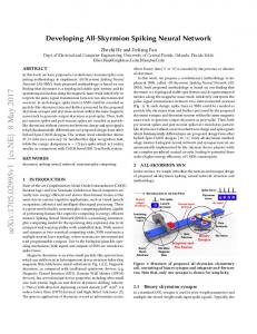
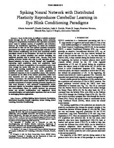
103
Figure 11: Speed improvement with vectorisation. We simulated the random network described in Appendix B with various numbers of neurons and compared it to a non-vectorised implementation (with loops, also written in Python). Vectorised code is faster for more than 3 neurons. postsynaptic neurons (i.e., targets of the event under consideration). Thus, if N is the number of neurons and p is the average number of synapses per neuron, then the interpretation overhead vanishes for differential equations (state updates) when N is large (Fig. 5) and for discrete events (spike propagation, plasticity) when p is large (Fig. 6). We previously showed that the Brian simulator, which implements these algorithms, is only about twice as slow as optimized custom C code for large networks (Goodman and Brette, 2008). In Fig. 11, we compared our vectorised implementation of a random network (Appendix B) with a non-vectorised implementation, also written in Python. Vectorised code is faster for more than 3 neurons, and is several hundred times faster for a large number of neurons. In principle, the algorithms could be further optimised by also vectorising discrete events over emitted spikes, but this would probably require some specific vector-based operations (in fact, matrix-based operations). An interesting extension would be to port these algorithms to graphics processing units (GPUs), which are parallel co-processors available on modern graphics cards. These are inexpensive units designed originally and primarily for computer games, which are increasingly being used for nongraphical parallel computing (Owens et al., 2007). The chips contain multiple processor cores (512 in the current state of the art designs) and parallel programming follows the SIMD model (single instruction, multiple data). This model is particularly well adapted to vectorised algorithms. Thus we expect that our algorithms could be ported to these chips with minimal changes, which could yield considerable improvements in simulation speed for considerably less human and financial investment than clusters. We have already implemented the state update part on GPU and applied it to a model fitting problem, with speed improvements of 50 to 80 on the GPU compared to single CPU simulations (Rossant et al., 2010). The next stage, which is more challenging, is to simulate discrete events on GPU. Another challenge is to incorporate integration methods that use continuous spike timings (i.e., not bound to the time grid), which have been recently proposed by several authors (D’Haene and Schrauwen, 2010; Hanuschkin et al., 2010). The first required addition is that spikes must be
17
communicated along with their precise timing. This could be simply done in a vectorised framework by transmitting a vector of spike times. Dealing with these spike timings in a vectorised way seems more challenging. However, in these methods, some of the more complicated operations occur only when spikes are produced (e.g. spike time interpolation) and thus may not need to be vectorised. Finally, we only addressed the simulation of networks of single-compartment neuron models. The simulation of a multicompartmental models could be vectorised over compartments, in the same way as the algorithms we presented are vectorised over neurons. The main difference would be to design a vectorised algorithm for simulation of the cable equation on the dendritic tree. As this amounts to solving a linear problem for a particular matrix structure defining the neuron morphology (Hines, 1984), it seems like an achievable goal.
Acknowledgements The authors would like to thank all those who tested early versions of Brian and made suggestions for improving it. This work was supported by the European Research Council (ERC StG 240132).
A
Spike container
The following Python code implements vectorised operations on a circular array (section 2.1.2) and the spike container structure described in section 2.4. Listing 1: Implementation of circular arrays and spike containers from scipy import * from numpy import * class CircularVector(object): def __init__(self, n): self.X = zeros(n, dtype=int) self.cursor = 0 self.n = n def __getitem__(self, i): return self.X[(self.cursor+i)%self.n] def __setitem__(self, i, x): self.X[(self.cursor+i)%self.n] = x def endpoints(self, i, j): return (self.cursor+i)%self.n, (self.cursor+j)%self.n def __getslice__(self, i, j): i0, j0 = self.endpoints(i, j) if j0>=i0: return self.X[i0:j0] else: return hstack((self.X[i0:], self.X[:j0])) def __setslice__(self, i, j, W): i0, j0 = self.endpoints(i, j) if j0>i0: self.X[i0:j0] = W elif j0