Preprint submitted to IMA Journal of Numerical Analysis (2013) Page 1 of 21
Interpolation with Variably Scaled Kernels M IRA B OZZINI† Dipartimento di Matematica e Applicazioni, Universit`a di Milano–Bicocca, Via Roberto Cozzi 53, 20125 Milano, Italy L ICIA L ENARDUZZI‡ CNR, IMATI Milano Department, via Bassini 15, 20133 Milano, Italy M ILVIA ROSSINI§ Dipartimento di Matematica e Applicazioni, Universit`a di Milano–Bicocca, Via Roberto Cozzi 53, 20125 Milano, Italy ROBERT S CHABACK¶ Institut f¨ur Numerische und Angewandte Mathematik Fakultt fr Mathematik und Informatik, Universit¨at G¨ottingen Lotzestraße 16-8, D–37073 G¨ottingen, Germany [Received on 28 August 2013] Within kernel–based interpolation and its many applications, it is a well–documented but unsolved problem to handle the scaling or the shape parameter. We consider native spaces whose kernels allow us to change the kernel scale of a d–variate interpolation problem locally, depending on the requirements of the application. The trick is to define a scale function c on the domain Ω ⊂ Rd to transform an interpolation problem from data locations x j in Rd to data locations (x j , c(x j )) and to use a fixed–scale kernel on Rd+1 for interpolation there. The (d + 1)–variate solution is then evaluated at (x, c(x)) for x ∈ Rd to give a d–variate interpolant with a varying scale. A large number of examples show how this can be done in practice to get results that are better than the fixed–scale technique, with respect to both condition and error. The background theory coincides with fixed–scale interpolation on the submanifold of Rd+1 given by the points (x, c(x)) of the graph of the scale function c. Keywords: positive definite radial basis functions; shape parameter; scaling.
1. Introduction A symmetric kernel K : Ω ×Ω → R defined on a domain Ω is very useful for a variety of purposes from interpolation or approximation to PDE solving, if certain nodes or centers x1 , . . . , xN ⊂ Rd are used to define kernel translates K(·, x j ) as trial functions. If the kernel is positive (semi–) definite, i.e. the kernel matrices with elements K(xi , x j ), 1 6 i, j 6 N are positive (semi–) definite for all choices of nodes, there is a native Hilbert ⊂ Rd
† Email:
[email protected]
‡
[email protected] § Corresponding ¶ Email:
author. Email:
[email protected] [email protected]
2 of 21
M. BOZZINI ET AL.
space H in the background in which the kernel is reproducing, i.e. f (x) = ( f , K(·, x))H for all x ∈ Ω , f ∈ H . The use of reproducing kernels in Hilbert spaces leads to various optimality properties and plenty of applications, but we leave details to the background literature [1, 6, 25, 23, 11]. If the kernel is translation–invariant on Rd , it is of the form K(x, y) = Φ (x−y) for all x, y ∈ Rd . In a geostatistical context, kernels are viewed as covariances of spatial ramdom variables, and then translation– invariant kernels are called stationary. If the kernel is radial, i.e. of the form K(x, y) = ϕ (∥x − y∥2 ) for a scalar function ϕ : [0, ∞) → R, the function ϕ is called a radial basis function. There also are compactly supported kernels which vanish outside the unit ball, e.g. the very useful Wendland kernels [24, 25]. Kernels on Rd can be scaled by a positive factor c by going over to the new kernel Kc (x, y) := K(x/c, y/c) for all x, y ∈ Rd .
(1.1)
In case of a radial kernel supported on the unit ball, the support of the scaled kernel now has support radius c. Large c increase the condition of kernel matrices, while small c let the translates turn into sharp peaks which approximate functions badly, if separated too far from each other. The choice of a scaling or shape parameter c of a kernel or radial basis function is a problem that is around for more than two decades [15, 20, 4, 5, 10, 13]. There are purely experimental reports on the behavior of kernel–based methods under scaling, and there are optimization techniques that try to find a good compromise between bad condition and good reproduction quality. A special case of scaling is the flat limit c → ∞ which is not considered here [9, 12, 18, 19, 21, 22]. Users would like to have the scale of a kernel translate vary with the translation. This means working with trial functions ϕ (∥x−x j ∥2 /c j ), 1 6 j 6 N in the radial case, but it is easy to come up with examples that let interpolation in the nodes fail for certain nonuniform choices of scale. This paper mimics the case of varying scales by letting the scale parameter be an additional coordinate. This allows varying scales without leaving the firm grounds of kernel–based interpolation. It turns out that this approach can be fully understood as the standard single–scale method applied to a certain submanifold of Rd+1 , and some numerical examples show that the method works quite satisfactorily in cases that are spoiled by excessive instability of the standard method. 2. Basics Let K be a positive definite kernel on Rd+1 . We assume readers to be familiar with this notion and with the standard examples of radial kernels, see e.g. [25]. Definition 1 If a scale function c : Rd → (0, ∞) is given, we can define a variably scaled kernel on Rd by Kc (x, y) := K((x, c(x)), (y, c(y))) for all x, y ∈ Rd . (2.1) Note that this definition is different from (1.1). We explain the differences below for special cases of radial kernels. The following is easy to prove.
INTERPOLATION WITH VARIABLY SCALED KERNELS
3 of 21
Theorem 1 If K is positive (semi–) definite, so is Kc . If K and c are continuous, so is Kc . If K is positive definite, interpolation of values f1 , . . . , fN on X := {x1 , . . . , xN } proceeds via solving a linear system Ac,X a = f ∈ RN with the kernel matrix Ac,X := (Kc (x j , xk ))16 j,k6N , which is positive definite. The coefficient vector a ∈ RN then allows the solution function to be written as sc,X, f (x) := 2.1
N
N
j=1
j=1
∑ a j Kc (x, x j ) = ∑ a j K((x, c(x)), (x j , c(x j ))).
(2.2)
Radial Kernels
If the kernel is radial, i.e. K(x, y) = ϕ (∥x − y∥22 ), then the kernel matrix entries are
ϕ (∥x j − xk ∥2 + (c(x j ) − c(xk ))2 ) and the interpolant is N
∑ a j ϕ (∥x − x j ∥22 + (c(x) − c(x j ))2 ).
sc,X, f (x) :=
j=1
It is identical to the standard kernel interpolant if the scale function is constant. 2.2
Power Kernels
Consider K to be a radial power kernel ϕ (r) = rβ . Then ( )β /2 Kc (x, y) = ∥x − y∥22 + (c(x) − c(y))2 ( )β /2 ∥x − y∥22 = |c(x) − c(y)|β + 1 (c(x) − c(y))2 is close to (but not identical) to a scaled multiquadric kernel. The interpolants take the form N
sc,X, f (x) :=
∑ aj
( )β /2 ∥x j − x∥22 + (c(x j ) − c(x))2
j=1
and are similar to scaled multiquadrics, while identical to power interpolants if the scale function is constant. 2.3
Multiquadrics
Consider K to be the standard multiquadric. Then ( )β /2 Kc (x, y) = ∥x − y∥22 + (c(x) − c(y))2 + 1 and the interpolants take the form N
sc,X, f (x) :=
∑ aj
( )β /2 . ∥x j − x∥22 + (c(x j ) − c(x))2 + 1
j=1
which can be seen as a variably scaled multiquadric.
4 of 21 2.4
M. BOZZINI ET AL.
Gaussian
Consider K to be the Gaussian. Then Kc (x, y) = exp(−∥x − y∥22 ) exp (−(c(x) − c(y))2 ) and the interpolants take the form N
sc,X, f (x) :=
∑ a j exp(−∥x j − x∥22 ) exp (−(c(x j ) − c(x))2 )
j=1
which can be seen as a superposition of Gaussians of the same scale but with varying amplitudes for evaluation. 2.5
Compactly Supported Radial Kernels
Consider K to be a radial kernel K(x, y) = ϕ (∥x − y∥22 ) with compact support in the unit ball of Rd+1 . Then the sparsity of the kernel matrix can be modified by the scale function c via ( ) Kc (x, y) = ϕ ∥x − y∥22 + (c(x) − c(y))2 . Since the interpolants take the form N
sc,X, f (x) :=
∑ a jϕ
( ) ∥x j − x∥22 + (c(x j ) − c(x))2 ,
j=1
the support radius can be influenced via c. 3. Theoretical Analysis The map C : x 7→ (x, c(x))
(3.1)
maps into a d-dimensional of A set X = {x1 , . . . , xN } ⊂ Ω of nodes goes into C(X) ⊂ C(Ω ) ⊂ C(Rd ) ⊂ Rd+1 . On Rd+1 and the point set C(X), interpolation by the unscaled kernel K takes place, and the resulting interpolant (2.2) takes the form Rd
submanifold C(Rd )
Rd+1 .
⊂ Rd
sc,X, f (x) = s1,C(X), f (x, c(x)) = s1,C(X), f (C(x)) with the interpolant s1,C(X), f at scale 1 of the data of f in the points (x1 , c(x1 )), . . . , (xN , c(xN )) of C(X). This means that in Rd+1 the kernel (2.1) is used, and if we project points (x, c(x)) ∈ Rd+1 back to x ∈ Rd , the projection of the kernel Kc on Rd+1 turns into a varying shape kernel on Rd whenever c(x) is not constant. Thus the analysis of error and stability of the varying–scale problem in Rd coincides with the analysis of a fixed–scale problem on a submanifold in Rd+1 . If C is assumed to be a diffeomorphism between Ω and C(Ω ), and if Ω is compact, one can see C(Ω ) as any other compact d–variate domain. The usual error and stability analysis focuses on fill distance h(X, Ω ) := sup min ∥x − y∥2 y∈Ω x∈X
INTERPOLATION WITH VARIABLY SCALED KERNELS
5 of 21
and separation distance q(X) :=
min ∥x − y∥2
X∋x̸=y∈X
in their standard definitions. These will transform with C accordingly, and will roughly be multiplied by a factor that scales with the norm of the gradient of c or the Lipschitz constant L of c. In particular, ∥C(x) −C(y)∥22 ∥C(x) −C(y)∥22
= ∥x − y∥22 + (c(x) − c(y))2 6 ∥x − y∥22 (1 + L)2 > ∥x − y∥22
shows that distances will blow up with C, letting separation distances never decrease, thus enhancing stability. But fill distances will also blow up, increasing the usual error bounds. This argument shows that one can successfully use the varying–scale (VSK) technique on points x j and xk that have ∥x j − xk ∥2 = q(X) > q(X), and this should be done for all close–by pairs of centers until one roughly gets that q(C(X)) ≈ h(X, Ω ) ≈ h(C(X),C(Ω )) holds, i.e. the transformed centers are approximately uniformly distributed. All of this is a special case of the following general principle. Given a kernel K : Ω × Ω → R and a bijective map C : Ω 7→ C(Ω ), the kernel KC (C(x),C(y)) := K(x, y) for all x, y ∈ Ω now acts on C(Ω ) and inherits the definiteness properties of K. This will also work “backwards”, i.e. for a bijective map onto Ω . This gives rise to two native spaces and their properties, i.e. f (x) = ( f , K(x, ·)) K(x, y) = (K(x, ·), K(y, ·)) for all x, y ∈ Ω and
g(u) = (g, KC (u, ·))C KC (u, v) = (KC (u, ·), KC (v, ·))C
for all u, v ∈ C(Ω ). Theorem 2 The native spaces for K and KC are isometric.
6 of 21
M. BOZZINI ET AL.
Proof: Functions f on Ω will map to functions C ( f ) on C(Ω ) via C ( f )(Cx) := f (x), and this map C is linear. Furthermore, C (K(·, x))(C(y)) = K(x, y) = KC (C(x),C(y)) and thus also C (K(·, x))(·) = KC (C(x), ·) hold. Thus we get K(x, y) = = = =
(K(x, ·), K(y, ·)) (C (K(·, x))(C(·)), C (K(·, y))(C(·))) KC (C(x),C(y)) (KC (C(x), ·), KC (C(y), ·))C
for the two inner products, and this means ( f , g) = (C ( f )(C(·)), C (g)(C(·))) = (C ( f ), C (g))C for all f , g in the span of all K(·, x), which are mapped to all C ( f ), C (g) in the span of all C (K(·, x)) = KC (C(x), ·). This proves that C is an isometry between the two native spaces. If we apply this to our special situation, we see that the native space for Kc on Ω is isometrically isomorphic to the native space for K1 on C(Ω ) for the C in (3.1). 4. Numerical Examples We now provide some examples that show the different roles of the variable scale parameter: it may affect both the stability and the accuracy. In 4.1 we will show how its appropriate choice enhances stability, while the rest of this section demonstrates that one can significantly improve the recovery quality, in particular by preserving shape properties in a much better way than for interpolation with constant scale. 4.1
Stability
4.1.1 Chebyshev Points . For univariate functions on Ω = [−1, +1], interpolation by polynomials should be done in Chebyshev points x j = − cos(π ( j − 1)/(N − 1)), 1 6 j 6 N rather than in equidistant points. But the fill distance of these points behaves like 1/N, while the separation distance behaves like 1/N 2 . If kernel–based methods are used, this leads to a very large condition in the kernel matrices, no matter which kernel is chosen. To√cope with this, we map the interval Ω = [−1, +1] ⊂ R to the semi– circle C(Ω ) ⊂ R2 via C(x) = (x, 1 − x2 ). Then the resulting points are equidistant, and we can work with a single–scale kernel in R2 for interpolation in C(X). The separation distance will now behave like 1/N like the fill distance. √ As a specific case, we chose the Gaussian kernel at fixed scale 0.1 · 2 and took 55 Chebyshev points to work with. For comparison, we also used 55 equidistant points. The L∞ errors for interpolating the Runge function f (x) = 1/(1 + 25x2 ) are given in Table 1(tabRunge). If there is no noise, the single scale methods are still superior. A possible explanation is that linear systems with badly conditioned kernel matrices and interpolation data from functions in the “native” Hilbert space have good approximate solutions based on a selection of columns, thus avoiding the influence of small separation distances. If additive random noise of maximal value ±0.001 is added, the above argument fails and the bad condition spoils the results seriously. Results for other kernels and point sets were similar. If there is no noise and the data are from a smooth function, single scale methods often work fine even if the condition is beyond the limit. The MATLAB
7 of 21
INTERPOLATION WITH VARIABLY SCALED KERNELS
Points and scaling equidistant, single scale Chebyshev, single scale Chebyshev, variable scale
Condition 5 · 1014 1 · 1016 8 · 105
no noise 7 · 10−5 1.1 · 10−5 1.3 · 10−4
0.001 noise 0.0331 1.4294 0.0012
Table 1. Interpolation of Runge function by Gaussians
backslash operator provides good approximate solutions in many cases. But as soon as noise and a bad condition of the single scale problem occur together, the variable scale tends to save the situation. In contrast to to polynomial interpolation, the equidistant case often is not seriously inferior to using Chebyshev nodes. 4.1.2 Monotonic Node Transformation in 1D. For scattered nodes −1 6 x1 < . . . < xN 6 1 in 1D one can find a transformation C that maps them into points z j ∈ R2 which are equidistant. If h is the fill distance of the given points, one can guarantee ∥z j+1 − z j ∥22 = (x j+1 − x j )2 + (c j+1 − c j )2 = 4h2 by choosing
√ c j+1 = c j +
4h2 − (x j+1 − x j )2 ,
starting with c1 = 0. This gives a monotonic sequence, and one can use piecewise linear interpolation to construct a continuous map C with C(x j ) = z j , 1 6 j 6 N of the form C(x) = (x, c(x)) with c being monotonic. Experiments with this strategy show a similar behavior like the previous example, but the non–differentiability of the map C spoils convergence rates. For a setting with 55 scattered points in [−1, +1], Figure 1(figC) shows the monotonic function c that increases sharply where there are close–by points, while it is flat over holes in the node set. Table 2(tabC) shows the corresponding conditions and errors, again for the Runge function. Readers should remember that the variable scale interpolation is a fixed scale interpolation along the curve in Figure 1(figC). The maximal errors are attained in all cases near the gap in the data near x = 0.1. The example shows that the current method (VSK) is more stable and robust. Points and scaling scattered, single scale scattered, variable scale
Condition 2.6 · 1016 3.8 · 108
no noise 1.3 · 10−5 0.0126
0.001 noise 0.0344 0.0125
Table 2. Interpolation of Runge function by Gaussians, scattered nodes
4.1.3 Cluster of data. We take N = 47 points xi ∈ [−1, 1] so that 41 nodes are equispaced in the interval and 6 close to 0.4, with mutual distance q = 10−4 . As c(x), we consider the skew-Gaussian [17] depicted in Fig. 2 t(x) := 2 · (x − 4.0005 · 10−1 )/(3.5 · 10−4 ) c(x) := exp(−(t 2 (x) + 5 · (1/π arctan(t(x) + 1) + 0.5)))
(4.1)
8 of 21
M. BOZZINI ET AL. 9
8
7
6
5
4
3
2
1
0 −1
−0.8
−0.6
−0.4
−0.2
0
0.2
0.4
0.6
0.8
1
FIG. 1. Monotonic function c for C(x) = (x, c(x))
0.035
0.03
0.025
0.02
0.015
0.01
0.005
0 0.399
0.3992
0.3994
0.3996
0.3998
0.4
0.4002
0.4004
0.4006
FIG. 2. C(x) = (x, c(x)) with some c(xi ) values
0.4008
0.401
9 of 21
INTERPOLATION WITH VARIABLY SCALED KERNELS
In Table 3, we show the condition numbers √ and the L∞ errors obtained interpolating the Runge function by the Gaussian kernel at fixed scale 0.1 · 2 and by the proposed technique. In Fig. 3 the plots of the absolute error for the two interpolants are depicted. Points and scaling cluster, single scale cluster, variable scale
Condition 3.5 · 1016 6.9 · 1010
error 6.02 · 10−5 9.4 · 10−6
0.001 noise 5.4 · 10−1 3.0 · 10−3
Table 3. Interpolation of Runge function by Gaussians, cluster nodes
−5
7
x 10
6
5
4
3
2
1
0 −1
−0.8
−0.6
−0.4
−0.2
0
0.2
0.4
0.6
0.8
1
FIG. 3. No noise case; absolute error for the classic case dotted; absolute error for the VSK-interpolant in full line
4.2
Enhancing reproduction quality
In this section, we deal with the problem of obtaining interpolants which reproduce faithfully the underlying functions. (see e.g. [3], [7]). In the following examples, we compare the classical interpolant provided by the C2 Wendland kernel with support radius 1 with the VSK interpolation provided by the d-variate C2 Wendland kernel with support radius µ (C(Ω ))1/d , where µ is the length or area of C(Ω ). 4.2.1 The logistic function. √
We consider the logistic function f (x) = (1 + 2 · exp(p(x)))−0.5 ,
(4.2)
where p(x) = −3 · (10 2x2 − 6.7). We take N = 11 nodes with a carefully chosen distribution in the interval Ω = [0, 1]. In particular, we want a higher density where the function changes more quickly and
10 of 21
M. BOZZINI ET AL.
a lower density where it is nearly constant. In this case we chose as variable scale c(x) the multiquadric interpolant sMQ of the given data (with δ = 0.03) multiplied by a tension coefficient. For this example,
c(x) = 2 · sMQ (x),
(4.3)
and its plot is shown in Fig. 4, together with the values c(xi ) marked.
2.5
2
1.5
1
0.5
0
−0.5
0
0.1
0.2
0.3
0.4
0.5
0.6
0.7
0.8
0.9
1
FIG. 4. C(x) = (x, c(x))
Note that the classical interpolant (Fig. 5) has near the right boundary an oscillation not consistent with the underlying function shape, while the VSK interpolant (Fig. 6) is a faithful recovery of (4.2). The absolute interpolation errors for the two interpolants are shown in Fig. 7. The L∞ errors are 2.5 · 10−2 for the fixed–scale case and 6.4 · 10−3 for the variable–scale case.
11 of 21
INTERPOLATION WITH VARIABLY SCALED KERNELS
1
0.8
0.6
0.4
0.2
0
0
0.1
0.2
0.3
0.4
0.5
0.6
0.7
0.8
0.9
1
FIG. 5. Classical Wendland interpolant full lined; logistic function dotted
1
0.8
0.6
0.4
0.2
0
0
0.1
0.2
0.3
0.4
0.5
0.6
0.7
0.8
0.9
1
FIG. 6. VSK-interpolant full lined; logistic function dotted
12 of 21
M. BOZZINI ET AL.
0.025
0.02
0.015
0.01
0.005
0
0
0.1
0.2
0.3
0.4
0.5
0.6
0.7
0.8
0.9
1
FIG. 7. Absolute error for the classic interpolant dotted; absolute error for the VSK interpolant full lined
4.2.2
The sigmoid function. We consider the function √ f (x, y) = (1 + 2 · exp(−3(9 x2 + y2 − 6.7)))−0.5
(x, y) ∈ Ω = [0, 1]2 ,
(4.4)
and a configuration of N = 89 nodes in Ω (see Fig. 8) with higher density where the function changes most. As in the previous example, we consider the variable scale (see Fig. 9, with marks on the transformed interpolation points)
c(x, y) = 2.5 sMQ (x, y),
(4.5)
where sMQ is the multiquadric interpolant to the given data with δ = 0.15. The classical interpolant and the VSK-interpolant are shown respectively in Figs. 10, 11 and the interpolation errors in Figs. 12, 13. The L∞ errors are 1.3 · 10−1 for the fixed–scale case and 2.5 · 10−2 for the variable–scale case.
INTERPOLATION WITH VARIABLY SCALED KERNELS
FIG. 8. Given nodes
13 of 21
14 of 21
M. BOZZINI ET AL.
3 2.5 2 1.5 1 0.5 0 −0.5 1 0.8
1 0.6
0.8 0.6
0.4 0.4
0.2
0.2 0
0
FIG. 9. C(x, y) = (x, y, c(x, y))
FIG. 10. Classical interpolation
15 of 21
INTERPOLATION WITH VARIABLY SCALED KERNELS
FIG. 11. sc,X, f (x)
0.2 0.15 0.1 1 0.05
0.9 0.8 0.7
0 0.6
0 0.5
0.2 0.4
0.4
0.3 0.6
0.2 0.1
0.8 1
0
FIG. 12. Absolute interpolation error; classical case
16 of 21
M. BOZZINI ET AL.
0.2 0.15 0.1 1 0.05
0.9 0.8
0
0.7
0
0.6 0.5
0.2 0.4
0.4
0.3 0.6
0.2 0.8
0.1 1
0
FIG. 13. Absolute error for the VSK-interpolant
4.3
Interpolant with optimal node configuration
In [8], the authors remarked that good node configurations X are those with q(X) ≈ h(X, Ω ). So our aim is to find a variable scale that transforms the given node set X = {xi }Ni=1 into a set C(X) satisfying q(C(X)) ≈ h(C(X),C(Ω )) ≈ h(X, Ω ). Let us consider the well–known humps and dips function by Franke [14] and N = 131 nodes belonging to a domain Ω1 ⊃ Ω = [0, 1]2 . The nodes are more dense in the zones of the maxima and of the minimum (see Fig. 14). We define the variable scale (see Fig. 15) as N
c(x, y) = ∑ pi (x, y),
(4.6)
i=1
where the functions pi (x, y) := (1/π · arctan(ai (x − xi )) + 1/2) · exp(−5 · (y − yi )2 ) increase more steeply at xi with a larger value of ai , if the local density of the data locations is large at xi . This choice allows us to increase the separation distance q where the node density is high without increasing too much the fill distance h, achieving or goal this way. In Fig. 16 we show the classical interpolant performed by using a Gaussian kernel with δ = 0.25 and in in Fig. 17 the VSK-interpolant. The corresponding interpolation errors are depicted in Figs. 18 and 19. The L∞ errors are 2.1 · 10−1 for the fixed-scale case and 4.2 · 10−2 for the variable–scale case.
INTERPOLATION WITH VARIABLY SCALED KERNELS
FIG. 14. Given nodes
17 of 21
18 of 21
M. BOZZINI ET AL.
1
0.8
0.6
0.4
0.2
0 1.5 1.5
1 1
0.5 0.5 0
0 −0.5
−0.5
FIG. 15. C(x, y) = (x, y, c(x, y))
1.4
1.2
1
0.8
0.6
0.4
0.2
0 0
0 0.2
0.2
0.4
0.4
0.6
0.6
0.8
0.8 1
1
FIG. 16. Classical interpolant
19 of 21
INTERPOLATION WITH VARIABLY SCALED KERNELS
1.4
1.2
1
0.8
0.6
0.4
0.2
0 0
0 0.2
0.2
0.4
0.4
0.6
0.6
0.8
0.8 1
1
FIG. 17. VSK-interpolant
0.25
0.2
0.15
0.1
0.05
0 0
0 0.2
0.2
0.4
0.4
0.6
0.6
0.8
0.8 1
1
FIG. 18. Absolute error for the classical interpolant
20 of 21
M. BOZZINI ET AL.
0.25
0.2
0.15
0.1
0.05
0 0
0 0.2
0.2
0.4
0.4
0.6
0.6
0.8
0.8 1
1
FIG. 19. Absolute error for the VSK-interpolant
5. Conclusions The examples show how the proper use of the variable scale kernel KC can lead to a more stable and better shape–preserving interpolant. In particular when the variable scale function c is chosen to depend on critical shape properties of the data, the interpolant reproduces the underlying phenomenon in a much more faithful way, and the interpolation error can be reduced in the critical regions to show a much more uniform behaviour in the whole domain. R EFERENCES Aronszajn N. (1950) Theory of reproducing kernels. Trans. Amer. Math. Soc., 68, 337–404. Bozzini M., Lenarduzzi L. (2005) Reconstruction of surfaces from a not large data set by interpolation. Rendiconti di Matematica, Serie VII, 25, 223–239. Bozzini M., Lenarduzzi L. (2003) Bivariate knot selection procedure and interpolation perturbed in scale and shape. Curve and Surface Design, T. Lyche, M. L. Mazure and L. Schumaker eds, 1–10. Bozzini M., Lenarduzzi L., Rossini M., Schaback R. (2004) Interpolation by basis functions of different scales and shapes. Calcolo, 41 (2), 77–87. Bozzini M., Lenarduzzi L., Schaback R. (2002) Adaptive interpolation by scaled multiquadrics. Advances in Computational Mathematics, 16 375–387. Buhmann M. D. (2003) Radial Basis Functions, Theory and Implementations. Cambridge University Press. Casciola G., Lazzaro D., Montefusco L. B., Morigi S.(2006) Shape preserving reconstruction using locally anisotropic radial basis function interpolants. Computer and Mathematics with Applications, 1, 1185–1198. De Marchi S., Schaback R., Wendland H. ( 2005) Near-optimal data-independent point locations for radial basis function interpolation. Adv. Comput. Math., 23(3), 317–330. Driscoll T. A., Fornberg B. (2002) Interpolation in the limit of increasingly flat radial basis functions. Comput. Math. Appl., 43, 413–422.
INTERPOLATION WITH VARIABLY SCALED KERNELS
21 of 21
Fasshauer G., Zhang J.G. (2007) On choosing optimal shape parameters for rbf approximation. Numerical Algorithms, 45, 345–368. Fasshauer G. (2007) Meshfree Approximation Methods with MATLAB, volume 6 of Interdisciplinary Mathematical Sciences. World Scientific Publishers, Singapore. Fornberg B., Wright G., Larsson L. (2004) Some observations regarding interpolants in the limit of flat radial basis functions. Computers & Mathematics with Applications, 47, 37–55. Fornberg B., Zuev J. (2007) The Runge phenomenon and spatially variable shape parameters in RBF interpolation. Comput. Math. Appl., 54 (3), 379–398. www.math.nps.navy.mil/ rfranke. Kansa E. J., Carlson R.E. (1992) Improved accuracy of multiquadric interpolation using variable shape parameters. Comput. Math. Appl., 24, 99–120. Iske A. (2004) Multiresolution Methods in Scattered Data Modelling, volume 37 of Lecture Notes in Computational Science and Engineering. Springer. Jamshidi A. A., Kirby M. J. (2009) Skew-radial basis function expansions for empirical modeling. SIAM J. Sci. Comp. 31, 4715–4743. Larsson E., Fornberg B. (2005) Theoretical and computational aspects of multivariate interpolation with increasingly flat radial basis functions. Comput. Math. Appl., 49,103–130. Lee Y.J., Yoon G.J., Yoon J. (2007) Convergence property of increasingly flat radial basis function interpolation to polynomial interpolation. SIAM J. Mathematical Analysis, 39, 470-488. Rippa S. (1999) An algorithm for selecting a good value for the parameter c in radial basis function interpolation. Adv. Comput. Math., 11 (2-3), 193–210. Schaback R. (2005) Multivariate interpolation by polynomials and radial basis functions. Constructive Approximation, 21, 293–317. Schaback R. (2008) Limit problems for interpolation by analytic radial basis functions. J. Comp. Appl. Math., 212, 127–149. Schaback R., Wendland H. (2006) Kernel techniques: from machine learning to meshless methods. Acta Numerica, 15, 543–639. Wendland H. (1995) Piecewise polynomial, positive definite and compactly supported radial functions of minimal degree. Advances in Computational Mathematics, 4, 389–396. Wendland H. (2005) Scattered Data Approximation. Cambridge University Press.