7Image interpolation by optimized spline-based kernels

7

Image interpolation by optimized spline-based kernels Atanas Gotchev, Karen Egiazarian, and Tapio Saramäki

In this chapter, we discuss the arbitrary scale image interpolation problem considered as a convolution-based operation. Use is made of the class of piecewise (spline-based) basis functions of minimal support constructed as combinations of uniform B-splines of different degrees that are very susceptible for optimization while being also very efficient in realization. Adjustable parameters in the combinations can be tuned by various optimization techniques. We favor a minimax optimization technique specified in Fourier domain and demonstrate its performance by comparing with other designs in terms of error kernel behavior and by interpolation experiments with real images. 7.1. Introduction Reconstruction of a certain continuous function from given uniformly sampled data is a common problem in many image processing tasks such as image enlargement, rotation, and rescaling. The problem is broadly known as image interpolation. CCD or CMOS arrays, the most used devices for recording digital images, create patterns of discrete pixels on rectangular grids. Many image processing applications, such as zooming, affine transforms, unwarping, require generating new pixels at coordinates different from the given grid. These new pixels can be generated by a two-stage procedure. First, a certain continuous function is reconstructed to fit the given uniformly sampled data and then it is resampled at the desired coordinates. The process is widely known as interpolation and, in order to be successful, the reconstruction (interpolation) functions have to be chosen properly. Some of the most commonly adopted interpolation models represent the continuous function under reconstruction as a discrete sum of weighted and shifted, adequately chosen, basis functions. This is the so-called linear or convolution-based interpolation. A more general framework considers the reconstruction functions as generators of shift-invariant spaces. This formalism allows making an elegant relation between the continuous function to be sampled or reconstructed and its

286

Interpolation by optimized spline kernels

approximation (projection) on a shift-invariant space in terms of its discrete representation (samples). Moreover, for this formalism, the approximation theory provides tools for quatifying the error between the function and its approximation. Among reconstruction functions generating shift-invariant spaces, B-splines have attracted special attention due to their efficiency and excellent approximation properties. Furthermore, piecewise polynomial functions expressed as linear combinations of B-splines of different degrees have been optimized to achieve even better approximation properties for shortest possible function’s support. In this chapter, we address the problem of image interpolation by optimized spline-based kernels. In Section 7.2, we state the interpolation problem in signal and frequency domains. We then describe the most general distortions caused by nonideal interpolation and quantitative measures for evaluating the performance of a particular interpolator. Further, in Section 7.3, we demonstrate how to design and analyze piecewise polynomial basis functions of minimal support which can be used in interpolation and projection tasks. The design is based on linear combinations of uniform B-splines of different degrees. We compare the basis kernels designed following different optimization criteria in terms of error kernel behavior and by interpolation experiments with real images. All our notations are for the one-dimensional (1D) case. While it helps to clarify the ideas in a simpler way with higher dimensions easy to generalize, it is also practical as in many applications separable interpolators as tensor product of 1D functions are preferred for their computational efficiency. 7.2. Basics of sampling and interpolation 7.2.1. Sampling Consider the most popular imaging system consisting of an optical system and digital image capturing device. The optical system (lens) focuses the scene on the imaging plane. Its performance depends, among other factors such as distance and focal length, on the finite aperture size. It determines the optical resolution limits. The optical transfer function (OTF), being the autocorrelation function of the aperture size [54], is also finite and hence cuts all spatial frequencies outside the region of its support. The next is the sampling device, transforming the captured image into pixels. In most modern digital imaging systems it is a kind of imaging sensor based on the principle of charge-coupled devices (CCDs) [54]. Then, the spatial resolution is limited by the spatial sampling rate, that is, the number of photo-detectors per unit length along a particular direction. The process of taking real scenes and converting them into pixels can be mathematically formalized by the processes of image acquisition and sampling. The optical system can be modeled as a spatial linear lowpass filter acting on the continuous two-dimensional signal. The output band-limited signal is then sampled at the sampling rate determined by the spatial distribution of the photo-detectors. While

Atanas Gotchev et al.

287

Image row ga (x)

−4

−3

−2

−1

0

1

2

3

4

1

2

3

4

3

4

(a) Sampled ga (x)comb(x) image row

−4

−3

−2

−1

0 (b)

Reconstructed ya (x) = [ga (x)comb(x)]∗ h(x) image row

−4

−3

−2

−1

0

1

2

(c) Figure 7.1. Sampling and reconstruction operations. (a) Initial continuous signal; (b) sampled at integers; (c) reconstructed by linear convolution (dashed-dotted line).

the optical system somehow blurs the signal, an insufficient sampling rate, caused by detectors spaced few and far between, can introduce aliasing. These two effects are inevitable. However, they have been well studied and are taken into account when designing modern imaging systems [14, 54]. Consider the one-dimensional function r(x) representing a true scene along the x-axis. As a result of optical blurring, modeled as linear convolution with a kernel s(x), we obtain another continuous function ga (x), smoother and bandlimited (Figure 7.1(a)): ga (x) = (r ∗ s)(x).

(7.1)

For the sake of simplicity we assume that the initial sampling grid is placed on the integer coordinates and generate the discrete sequence g[k] = ga (x). In continuous time it can be modeled by the product ga (x) comb(x), where comb(x) =

∞ !

k=−∞

δ(x − k).

(7.2)

The resulting impulse train is a sum of integer-shifted ideal impulses weighted by the signal values at the same coordinates g p (x) = ga (x)

∞ !

k=−∞

δ(x − k) =

∞ !

k=−∞

g[k]δ(x − k).

(7.3)

288


Figure 7.1(b) illustrates the sampling process. The blurring effect can be quantified as the difference between the functions r(x) and ga (x) measured by the L2 error norm "

"

2 = "r − ga "L2 = εblur

#∞

−∞

$

%2

r(x) − ga (x) dx.

(7.4)

It is expressible in the Fourier domain as 2 εblur =

#

& & & & &1 − S(2π f )&2 &R(2π f )&3 df ,

(7.5)

where R(2π f ) is the Fourier transform of the initial signal r(x) and S(2π f ) is the frequency response of the (optical) blurring system. The effect of sampling is well studied in the Fourier domain. The Fourier transform G p (2π f ) of the product ga (x) comb(x) contains the original spectrum of ga (x) and its replications around multiples of 2π [43], G p (2π f ) =

∞ !

n=−∞

$

%

Ga 2π( f − n) ,

(7.6)

where Ga (2π f ) is Fourier transform of the blurred continuous signal ga (x). Any overlap of the replicated spectra can cause a degradation of the original spectrum. The effect is known as aliasing. 7.2.2. Interpolation Generally speaking, the role of the interpolation is to generate some missing intermediate points between the given discrete pixels. First, based on the existing discrete data, a continuous signal is generated and then, the desired interpolated samples are obtained by resampling it at the desired coordinates. In this general setting, the interpolation factor is arbitrary, not necessarily an integer, not even a rational number. In most cases, the continuous (analog) model fitting is performed by convolving the samples with some appropriate continuous interpolating kernel [62], as illustrated in Figure 7.1(c). The interpolation does not recover the original scene continuous signal itself. In most cases one starts directly with discrete data and does not know the characteristics of the optical system nor the sampling rate and the effects introduced by the sampling device. What one can do is to try matching a continuous model that is consistent with the discrete data in order to be able to perform some further continuous processing, such as differentiation, or to resample the fitted continuous function into a finer grid. Within this consideration, interpolation does not deal with inverse problems such as deconvolution, although some knowledge about the acquisition and sampling devices could help in the choice of the interpolating function [66].


289 h(x − 1)

ya (x)

∆

h(x) h(x + 1)

nl nl − 1 ∆(l − 2) ∆(l − 1) ∆l

1

µl

nl + 1 ∆(l + 1) µl+1

g[k] - initial samples

y[l] - new samples

Figure 7.2. Interpolation problem in signal domain. White circles represent initial discrete sequence g[k] with sampling ratio 1. Black circles represent new sequence y[l] taken with smaller sampling interval ∆ from continuous function ya (x).

7.2.2.1. Interpolation problem in signal domain Assume that there exist given discrete data g[k] defined on a uniform grid κ ≡ {0, 1, 2, . . . ,Lin −1}, k ∈ κ, with sampling step equal to unity, as shown in Figure 7.2. The g[k]’s can represent, for example, the pixel intensities in an image row or column. Furthermore, it is supposed that the data have been taken from a certain continuous function ga (x). The general interpolation problem is then to generate a new sequence y[l] with sampling points located at new points between the existing samples g[k] with the goal being to yield an image (row or column) with an increased number of pixels (a magnified, a zoomed in image). The new sequence y[l] can be generated by first fitting an approximating continuous function ya (x) to the given sequence g[k] and then resampling it at the desired new sampling points, as shown in Figure 7.2. For the uniform resampling, y[l] = ya (xl ) = ya (l∆) with ∆ < 1. The function ya (x) approximating the original continuous signal ga (x) can be generated by a linear, convolution-type model: ya (x) =

! k

(7.7)

g[k]h(x − k).

Here, h(x) is a continuous convolution kernel (interpolation filter) mapping the discrete data onto the continuous model function ya (x). The only information that we have about the continuous function ga (x) is conveyed by the samples g[k] and a natural assumption is that g[k] = ga (k). We require the same from the new function ya (x), that is, for all k0 ∈ κ, ya (k0 ) = g[k0 ]. This requirement imposes the so-called interpolation constraint for the kernel h(x) as follows: $ %

ya k0 =

! k

$

%

$

%

⎧ ⎨1,

g[k]h k0 − k !⇒ h k0 − k = ⎩ 0,

for k = k0 , otherwise.

(7.8)

290


The interpolation kernel should behave like h(k) = δ(k), where δ(k) is the Kroneker symbol. We say that the kernel h(x) is interpolating. A more general model can be stated. Consider another convolution kernel ϕ(x) which generates the approximating function ya (x): ya (x) =

! k

d[k]ϕ(x − k).

(7.9)

The model coefficients d[k] do not (necessarily) coincide with the initial signal samples g[k] and the reconstruction kernel ϕ(x) is not required to pass through zeros for the integer coordinates (noninterpolating kernel). Still, we require ya (k0 )= g[k0 ] for all k0 ∈ κ, that is, $ %

ya k0 =

! k

$

%

d[k]ϕ k0 − k = g[k0 ].

(7.10)

Equation (7.10) determines uniquely the model coefficients. It is in fact a discrete convolution between two sequences: the model coefficients and the interpolation function ϕ(x) sampled at integers. Denote it by p[k] = ϕ(k) and write the convolution (7.10) in z-domain: Ya (z) = D(z)P(z),

(7.11)

where Ya (z), D(z), and P(z) are the z-transforms of ya (k) = g[k], d[k], and p[k], respectively. The sequence of model coefficients is obtained by a recursive digital filtering, as follows: D(z) =

Ya (z) G(z) = . P(z) P(z)

(7.12)

Provided that ϕ is a finitely supported and symmetric function (as in most cases of interest), its sampled version is a symmetric finite length sequence p[k]. The recursive digital filter 1/P(z) is regarded as corresponding to an infinite discrete sequence, (p−1 )[k] being the convolution inverse of the sequence p[k], that is, $

%

p ∗ p−1 [k] = δ[k].

(7.13)

In time domain the filtering (7.12) can be formally expressed as $

%

d[k] = p−1 ∗ g [k].

(7.14)

Consequently, the interpolation approach (7.9) involves the preliminary filtering step (7.14) to get the model coefficients d[k]. It is not a costly operation and


291

for a large class of reconstruction kernels, can be realized through an efficient IIR filtering [62, 69, 70, 72]. The benefit is that the function ϕ(x) can be chosen with better properties, in particular it can be nonoscillatory by contrast to interpolating function h(x). The model (7.9) can be brought to the model (7.7) by replacing d[k] in (7.9) with (7.14), ya (x) =

!$ k

%

p−1 ∗ g [k]ϕ(x − k) =

! k

$

%

g[k] p−1 ∗ ϕ (x − k).

(7.15)

The convolution h(x) =

!$ k

%

p−1 [k]ϕ(x − k)

(7.16)

results in an infinitely supported interpolating kernel having the following frequency response: Φ(2π f ) H(2π f ) = $ j2π f % , P e

(7.17)

where Φ(2π f ) is the continuous frequency response of ϕ(x) and P(e j2π f ) = P(z)|z=e j2π f . After building the continuous model as given by (7.7) or (7.9), it is resampled at new discrete points to obtain y(l) = ya (xl ). Here, the current output coordinate xl can be expressed as xl = nl + µl , where nl = ⌊ xl ⌋ is the coordinate (integer) of g[nl ], occurring just before or at xl . The interval µl = xl − nl , in turn, is a fractional interval in the range 0 ≤ µl < 1. Given nl and µl , the current output pixel can be generated following (7.7): y[l] =

! * k

+ $

%

g nl − k h k + µ l .

(7.18)

From this equation, the interpolation kernel h(x) can be interpreted also as a filter with varying impulse response that depends on the value of µl . That is why in the literature it appears under different names such as interpolation kernel, interpolation filter, fractional delay filter, and reconstruction filter, emphasizing some of its properties [77]. Despite its different names, the kernel should be as follows. (i) The kernel is desired to be symmetrical to avoid introducing phase distortions. (ii) The kernel’s support should be as short as possible for the desired interpolation accuracy. This decreases the computational complexity, especially for highdimensional cases. Regarding the model (7.9), the support of the reconstruction function ϕ is envisaged. In fact, for this model, the cardinal interpolation function is infinitely supported because of the IIR term, but still the computational complexity would be sufficiently low for short-length kernels.

292


(iii) The kernel should ensure good closeness of the approximating function ya (x) to the unknown function ga (x). This closeness can be measured via different measures, that is, (1) in frequency domain, thus invoking the terms of passband preservation and stopband attenuation [55, 77]; (2) by the kernel’s approximation order, measuring its capability to reproduce polynomials up to some degree M and characterizing the rate of decay of the approximation error when the sampling interval tends to zero [62, 63]. These terms and some adequate measures of goodness will be discussed in detail later in this chapter. 7.2.2.2. Interpolation problem in frequency domain The Fourier transform of the initial sequence g[k] is the periodical version of Ga ( f ): $

%

G e j2π f =

∞ !

n=−∞

$

%

Ga 2π( f − n) .

(7.19)

The continuous function ya (x), as given by (7.7), can be expressed in the frequency domain as $

%

Ya (2π f ) = H(2π f )G e j2π f = H(2π f )

∞ !

k=−∞

$

%

Ga 2π( f − k) .

(7.20)

See Figure 7.3 for an illustration of the effects of sampling and reconstruction in frequency domain. Sinc (ideal) reconstruction kernel. In the ideal case it is desired that Ya (2π f ) = Ga (2π f ). The classical assumption is that the signal ga (x) is band-limited (or had been filtered to be band-limited), that is, Ga (2π f ) is zero for higher frequencies. The classic Shannon theorem [57] states that a band-limited signal ga (x) can be restored from its samples taken at integer coordinates, provided that Ga (2π f ) is zero for | f | > 1/2. Otherwise the sampling introduces aliasing. The interpolation starts where sampling has finished: from the discrete sequence g[k] having a periodical Fourier representation. The interpolation cannot restore frequencies distorted by aliasing. The best it can do is to try to restore a continuous function yideal (x) having Fourier transform ⎧ $ % ⎪ ⎪ ⎨G e j2π f ,

Yideal (2π f ) = ⎪ ⎪ ⎩0,

1 for 0 ≤ f ≤ , 2 1 for f > , 2

(7.21)


293 0

Magnitude (dB)

−10 −20 −30 −40 −50 −60 −70 −80

0

0.5

1 1.5 2 Normalized frequency

2.5

3

|H(2π f )|

Hideal (2π f ) Figure 7.3. Effects of sampling and reconstruction in frequency domain. |G(e j2π f )| is replicated version of |Ga (2π f )|. Hideal (2π f ) (solid line) is finite supported in frequency domain, while |H(2π f )| (dashed line) has side lobes.

and hope that the sampling has introduced no (little) aliasing. Hence, the ideal interpolation (reconstruction) is achieved by the filter ⎧ ⎪ ⎪ ⎨1,

Hideal (2π f ) = ⎪

⎪ ⎩0,

1 for 0 ≤ f ≤ , 2 1 for f > . 2

(7.22)

In the signal domain, the ideal filter is inversely transformed to the sinc function hideal (x) =

#∞

−∞

Hideal (2π f )e− j2π f x df =

sin(πx) = sinc(x). πx

(7.23)

The reconstruction equation for the case of the sinc reconstruction function is yideal (x) =

∞ !

k=−∞

g[k] sinc(x − k).

(7.24)

In the real world, the ideal filtering cannot be achieved since the sinc reconstruction function is infinitely supported (note the summation limits in (7.24)). Even if the initial signal g[k] is given on the finite interval 0 ≤ k ≤ M − 1 only, to reconstruct the continuous function ga (x) in this interval, we need an infinite summation. For signals given on a finite interval of M samples, the sinc-function should be replaced by a discrete the sinc-function sincd(x) = sin(πx)/(M sin(πx/M)) which is an ideal, to the accuracy of boundary effects, interpolator of discrete

294


signals with finite support [82, 83]. This interpolation method is considered in Chapter 8. Nonideal reconstruction kernels. Finitely supported nonideal reconstruction kernels have infinite frequency response. Being attractive due to their easier implementation, they never cancel fully the replicated frequencies above the Nyquist rate. Figure 7.3 illustrates this effect. An explicit relation between the output discrete signal y[l] and the input signal g[k] can be established, assuming a uniform resampling of ya (x) with the resampling step ∆ < 1 (finer than the initial one, i.e., the resampling generates more pixels). The Fourier transform of the output signal y[l] can be expressed in the following forms:

$

%

Y e j2π f ∆ = $

Y e

j2π f ∆

%

∞

-

∞

-

1 ! n Ya 2π f − ∆ n=−∞ ∆ -

-

1 ! n = H 2π f − ∆ n=−∞ ∆

..

$

..

,

(7.25) %

G e j2π( f −n/∆) .

(7.26)

This clarifies that the interpolation process generates some frequency regions which are mirrors of the passband frequency region with respect to 2π/∆. As an example, let us take the simplest interpolator, the so-called nearest neighbor. Practically, this interpolator repeats the value at the closest integer coordinate to the needed new coordinate. Following (7.7), this repetition is modeled by a convolution between the given discrete sequence and a rectangular reconstruction function having support between −1/2 and 1/2. The Fourier transform of this reconstruction function is a sinc function in the frequency domain, that is, sin(π f )/π f . It has high magnitude side lobes that overlap (not suppress!) the periodical replicas in the product (7.20) and in (7.26), respectively. Moreover, it is not flat for the frequencies below half the sampling rate and it attenuates considerably the true (passband) frequencies of the original signal resulting in visible blur. The two extreme cases, namely, sinc and nearest neighbor interpolators suggest directions for improving the performance of finite support interpolators. With some preliminary knowledge about the frequency characteristics of ga (x), the interpolator h(x) can be designed in such a way that its frequency response suppresses effectively the undesired components of the interpolated signal. This is equivalent to designing some application-specific optimized approximation of the ideal reconstruction filter in frequency domain. 7.2.2.3. Interpolation artifacts Before studying some quantitative measures of interpolators’ performance let us summarize qualitatively the distortions caused by nonideal interpolators.


295

Ringing. Ringing is a result of the oscillatory type of interpolators combined with the Gibbs effects due to the finite terms approximation of continuous functions in Fourier domain. Ringing effect occurs even for the ideal sinc interpolators realized in Fourier domain. Actually, those are not true artifacts since they can arise together with the perfect recovering of the initial samples [82]. Blurring. Blurring is a result of the nonideality of the reconstruction function in the passband. Instead of preserving all frequencies in this region, nonideal interpolators suppress some of them, especially in the high-frequency area (close to half the sampling rate). As a result, the interpolated images appeared with no sharp details, that is, blurred. Aliasing. Aliasing is an effect due to improper sampling. This is the effect of the appearing of unwanted frequencies (hence the term aliasing) as a result of the repetition of the original spectrum around multiples of the sampling rate. The aliasing artifacts resulting from insufficient sampling may appear as Moiré patterns. For small images, they may be hardly noticeable, but after interpolation on a finer grid they can become visible. Imaging. This is the counterpart of aliasing, though the term “imaging” is somehow confusing. Consider the simple case of sampling rate expansion by an integer factor of L. It can be accomplished by first inserting L − 1 zeros between the given samples (up-sampling) and then smoothing the new sequence with a digital filter. The up-sampling causes “stretching” of the frequency axis [43]. As a result, in the passband the original spectrum appears together with its L − 1 “images.” The role of the smoothing filter is to remove these unwanted frequencies. Following the model (7.7), we first apply the reconstruction operation (fitting the continuous model ya (x)) and subsequently the resampling. Assuming this model, unwanted frequencies can interfere into the passband during the process of resampling as a result of nonsufficient suppression of the frequency replicas during the previous step of continuous reconstruction. Hence, this effect can be again characterized as aliasing, and we will use this term in order not to confuse “imaging” with digital images. The effects of possible sampling-caused and reconstruction-caused aliasings are almost undistinguishable since they appear simultaneously (and with blurring) in the resampled image. The reconstruction-caused aliasing effect is emphasized for short-length kernels (i.e., nearest neighbor or linear) and appears in the form of blocking (pixelation) in the magnified image [62, 82]. 7.2.2.4. Interpolation error kernel There are two sources of errors caused by the nonideality of the reconstruction kernel to be quantified. First, there is the nonflat magnitude response in the passband (causing blurring) and second, there is the nonsufficient suppression of the periodical replicas in the stopband (causing aliasing). As the blurring and aliasing errors both superimpose into the resampled image, it is good to have an integral measure for both of them. Such a measure would play a substantial role in optimizing and comparing different interpolators. We review the interpolation error

296


kernel as it has appeared in the work of Park and Schowengerdt [48]. Then, based on some approximation theory presumptions, we review a generalized form of this kernel, appropriate for the interpolation model (7.9), see [10, 64]. Sampling and reconstruction (SR) blur. Park and Schowengerdt [48] have investigated the influence of the phase of sampling on the sampling and reconstruction accuracy. Return to image acquisition model (7.1)-(7.2) and insert an additional parameter u, showing the relative position of the sampling device with respect to the function s(x): ga (x − u) = (r ∗ s)(x − u).

(7.27)

Sampling at integers and reconstructing by a continuous interpolation function give ya (x, u) =

∞ !

k=−∞

ga (n − u)h(x − k).

(7.28)

Here, the reconstructed function also depends on the sampling phase and it is not simply a function of the difference x − u. The error between g(x − u) and y(x, u), called by the authors sampling and reconstruction (SR) blur, is a function of u as well: 2 (u) = εSR

#∞

−∞

$

%2

ga (x − u) − y(x, u) dx.

(7.29)

One can observe that the phase-dependent SR error is a periodic function of u with a period of unity and hence it can be represented as the Fourier series 2 εSR (u) =

∞ !

am e j2πum ,

(7.30)

m=−∞

where am =

#1 0

2 εSR (u)e− j2πum du.

(7.31)

The coefficient a0 plays the most important role since it quantifies the average value of the SR blur. It can be regarded as the expectation of the random error, depending on the arbitrary sampling phase. It can be obtained by taking the SR blur in frequency domain (Parseval’s equality) 2 (u) = εSR

#∞ / ! ∞ $ −∞

×

/

k=−∞

∞ !

n=−∞

$

%

$

%

$

%

δk − H(2π f ) Ga 2π( f − k) e j2πku ∗

%

∗

δn − H (2π f ) Ga 2π( f − n) e

0

− j2πnu

0

(7.32) df


297

and integrating over u a0 =

#∞

−∞

$

∞ ! $

∞ !

k=−∞ n=−∞

%

$

δk − H(2π f ) Ga 2π( f − k)

∗

%

∗

$

× δn − H (2π f ) Ga 2π( f − n)

%

#1 0

e

%

j2π(k−n)u

(7.33) du df .

After some simplifications we get 1

2

2 E εSR = a0 =

#∞

& & 3 & 4 $ % & &Ga (2π f )&2 1 − 2 Re H(2π f ) + &H(2π f )&2

−∞

&2 ! & $ %& &Ga 2π( f − k) &2 df

&

+ &H(2π f )&

k̸=0

#∞ 5 & &$ & %& &Ga (2π f )&2 & 1 − H(2π f ) &2 = −∞

(7.34)

6 & &2 ! & $ %&2 & & & & + H(2π f ) Ga 2π( f − k) df . k̸=0

The first term in the summation inside the integral is the error introduced by the nonideality of the reconstruction kernel (i.e., blurring term), while the second term represents the aliasing error due to the nonideality of the reconstruction kernel for the replicated frequencies. By changing the variable, this term can be rewritten in an equivalent form as follows: #∞

−∞

& & !& $ %& &H(2π f )&2 &Ga 2π( f − k) &2 df =

k̸=0

#∞

−∞

& & !& $ %& &Ga (2π f )&2 &H 2π( f − k) &2 df .

(7.35)

k̸=0

The average SR blur takes a very compact form which separates the influence of the reconstruction kernel and the initial signal 1

2

2 E εSR =

where &

#∞

−∞

&

&2

η2 (2π f )&Ga (2π f )& df , &2

η2 (2π f ) = &1 − H(2π f )& +

!& $ %& &H 2π( f − k) &2 .

(7.36)

(7.37)

k̸=0

Here, the nonnegative kernel η2 quantifies the amount of errors introduced by the reconstruction kernel.

298

Interpolation by optimized spline kernels The total SR error is 2 εSR (u) = εS2 (u) + εR2 (u) + φ(u),

(7.38)

where εS2 =

#∞

εR2 =

#∞

φ(u) =

−∞

−∞

!

& & !& $ %& &G(2π f )&2 &H 2π( f − k) &2 df , k̸=0

& & & & &G(2π f )&2 &1 − H(2π f )&2 df ,

(7.39)

am e j2πmu .

m̸=0

The term εS2 is regarded as the error due to insufficient sampling. It is also this term that is responsible for introducing the aliasing errors if the reconstructed signal is resampled into a finer grid. The term εR2 shows the error contribution of a reconstruction function which is different from unity in the frequency areas of significant signal energy. The last, namely, the sampling phase-dependant term φ(u), determined by the higher harmonics in the Fourier series (7.30), is a zero mean 7 2 random variable with variance 2 ∞ m=1 |am | . It is always zero if the initial signal is essentially band-limited and sufficiently sampled [48]. For a particular nonbandlimited signal, equations for am should be written and calculated (numerically). Many authors prefer just to study the behavior of the averaged error for different signals and different reconstruction kernels [40, 48, 49, 56]. A generalization of the error kernel (7.37) can be obtained based on the reconstruction model (7.9). Write the cardinal interpolation kernel (7.16) in frequency domain Φ(2π f ) Φ(2π f ) $ %, H(2π f ) = $ j2π f % = 7∞ P e k=−∞ Φ 2π( f − k)

(7.40)

7

where P(e j2π f ) = ∞ k=−∞ Φ(2π( f − k)) is the frequency response of the sampled version p(k) of the reconstruction function ϕ(x). The error kernel (7.37) becomes $

%

& &2 ! & & & Φ 2π( f − k) &2 & Φ(2π f ) & & $ & + & $ % % 1 − η2 (2π f ) = & & P e j2π f & k̸=0 & P e j2π( f −k) &

& $ j2π f % &2 7 & $ %&2 &P e − Φ(2π f )& + k̸=0 &Φ 2π( f − k) & = & $ %& &P e j2π f &2

(7.41)


299

2

Error kernel

1.5 1 0.5 0 −0.5

0.1 0.2 0.3 0.4 0.5 0.6 0.7 0.8 0.9 Normalized frequency Sinc Linear

1

Cubic B-spline of third degree

Figure 7.4. Error kernel for four classical interpolators.

or has the following equivalent form [64]: η2 ( j2π f ) =

&7 &

k̸=0 Φ

& $ %&2 7 %&2 2π( f − k) & + k̸=0 &Φ 2π( f − k) &

$

&7∞ &

k=−∞ Φ

$

%&2 2π( f − k) &

.

(7.42)

Figure 7.4 shows the error kernel for the ideal (sinc) interpolator and for the probably most used interpolating linear and cubic interpolators, and for the noninterpolating B-spline interpolator of third degree [33, 48, 49, 62]. The improvement of cubic versus linear interpolator is achieved thanks to the longer support and the higher degree. The B-spline has the same degree as the cubic convolution interpolator and the improvement is achieved thanks to the noninterpolating model applied. B-spline basis functions are described in the next section. The role of the error kernel will be additionally highlighted from an approximation theory point of view. How to compute the error kernel. Since the class of symmetrical, finitely supported interpolators is of major interest, we give some practical directions regarding how to compute the error kernel (7.42) for this class. Assume the function ϕ(x) is supported over the interval [−(N + 1)/2, (N + 1)/2] and is symmetrical, that is, ϕ(−x) = ϕ(x). Its sampled version, given by the sequence p(k) = ϕ(x)|x=k , is also symmetrical and has 2⌊ N/2⌋ + 1 nonzero terms. The Fourier transform of this sequence is given by &

P(z)&z=e j2π f = ϕ(0) + 2

⌊ N/2 !⌋

k=1

ϕ(k) cos(2πk f ).

(7.43)

300

Interpolation by optimized spline kernels For such a reconstruction function ϕ(x), (7.41) can be simplified,

η2 (2π f ) =

$ $

=

$ $

=

%

%2

P e j2π f − Φ(2π f ) P e

$ $

P

P e

%%2 j2π f

e j2π f

$ $

%%2

$

+

7

k̸=0 %%2 j2π f

$ $

Φ 2π( f − k)

%%2

% $ %2 7 $ $ %%2 − 2P e j2π f · Φ(2π f )+ Φ(2π f ) + k∈Z∗ Φ 2π( f − k) $ $ j2π f %%2 − 2P

$

e j2π f

%

P e

· Φ(2π f ) + $ $ j2π f %%2

P e

7∞

k=−∞

$ $

Φ 2π( f − k)

%%2

.

(7.44)

Although it is an infinite sum, the last term in the numerator can be calculated rather easily, realizing that it is the Fourier transform of the function ϕ(x) continuously convolved by itself and subsequently sampled. The autoconvolution (which is in fact an autocorrelation) is also symmetrical and has a compact support of 2N + 2. Hence, only N cosine terms take part in the considered infinite sum ∞ ! $ $

k=−∞

Φ 2π( f − k)

%%2

= (ϕ ∗ ϕ)(0) + 2

N !

k=1

(ϕ ∗ ϕ)(k) cos(2πk f ).

(7.45)

The algorithm for calculating the error kernel can be summarized as follows. (1) Calculate the Fourier transform Φ(2π f ) of the continuous kernel ϕ(x). (2) Calculate the Fourier transform P(e j2π f ) of the discrete kernel p(k) = ϕ(x)|x=k , as given by (7.43). (3) Calculate the autocorrelation function of the symmetrical continuous function ϕ(x), aϕ (x) = (ϕ ∗ ϕ)(x) at integer coordinates k : a[k] = aϕ (x)|x=k . (4) Find the Fourier transform of the sequence a(k), according to (7.45). (5) Calculate the kernel (7.44). 7.2.3. Shift-invariant function spaces and generating bases The model (7.9) has, in fact, a wider scope than the interpolation we have used it for. For an arbitrary choice of the model sequence d[k], the functions ϕ(x − k) span a vector space. The function space reformulation of the model (7.9) allows considering other schemes for obtaining the sequence d[k], apart from the simple interpolation [10]. Consider the following shift-invariant function space V (ϕ) that is a closed subspace of L2 and generated by a function ϕ as 5

V (ϕ) : gV (x) =

∞ !

k=−∞

d[k]ϕ(x − k) : c ∈ l

2

6

.

(7.46)


301

Any function from the space V (ϕ) can be represented as a convolution between a discrete set of coefficients and the generating function ϕ. In other words, the integer shifts of ϕ form a basis for the space V (ϕ) and the coefficients d[k] are regarded as coordinates of the function gV (x) with respect to the given basis. The generating function has to be chosen in an appropriate manner in order to ensure that the space V (ϕ) is a closed subspace of L2 , that is, ϕ must form a Riesz basis [3]. By definition, the family of basis functions ϕ(x − k) forms a Riesz basis if there exist two constants B > A > 0 such that A∥d∥2l2

" ∞ "2 " ! " " " ≤" d[k]ϕ(x − k)" ≤ B ∥d ∥2l2 . " " 2 k=−∞

(7.47)

L

The upper bound ensures that V (ϕ) is a well-defined subspace of L2 , while the lower bound provides that it is a closed subspace of L2 . A function in V (ϕ) is entirely described by the discrete-time sequence d[k]. Any function ga (x) ∈ L2 can be approximated by a function in V (ϕ). The interpolation is the simplest way of approximating ga (x) as was discussed in the previous sections. The least squares (LS) approximation is achieved by a preliminary filtering with an analysis (projecting) function. Since V (ϕ) is closed, the LS approximation g8a (x) exists and it is equal to the orthogonal projection of ga (x) into V (ϕ). In general, the basis ϕ(x − k) is not orthogonal, but only linearly independent. Then, the orthogonal projection of ga (x) ∈ L2 into V (ϕ) is obtained by g8a (x) =

∞ !

d[k]ϕ(x − k),

(7.48)

ga (τ)ϕ(k 8 − τ)dτ.

(7.49)

k=−∞

where d[k] =

#∞

−∞

Here, ϕ(x) 8 is the dual (biorthogonal) basis of ϕ. As it belongs to the same space V , it can be represented as a linear combination of the generating basis ϕ as well. Moreover, its coordinate coefficients are merely the autocorrelation sequence of ϕ, defined at the integer values as ϕ8 ∈ V (ϕ), $

%

ϕ(x) 8 = (a)−1 ∗ ϕ (x),

a[k] =

#∞

−∞

ϕ(τ)ϕ(τ − k)dτ.

The proof of this relation can be found, for example, in [3].

(7.50)

302


Taking the Fourier transform of (7.50) we obtain the dual basis in Fourier domain 8 Φ(2π f)=

Φ(2π f ) Φ(2π f ) $ % = 7 & & . ∞ &Φ(2π( f − n))&2 A e j2π f n=−∞

(7.51)

7.2.4. Approximation theory impact

In order to quantify the approximation error between ga (x) and its approximation as a function of the sampling step ∆ we write a scale-dependent convolution-based signal expansion: y∆ (x) =

!

-- .

d[k]ϕ

k

.

x −k . ∆

(7.52)

This is an expansion of a signal belonging to the space generated by the reconstruction function ϕ parameterized by the sampling (scale) parameter ∆, 9 -- .

V∆ = span ϕ k∈Z

x −k ∆

.:

(7.53)

.

The expansion coefficients d[k] can be obtained either by interpolation or by projection of ga (x) onto V∆ , for example, LS approximation. In both cases, the approximation theorists have been interested in quantifying the error between ga (x) and y∆ (x) as a function of the decreasing and eventually vanishing sampling step ∆ represented in the form 2

1

2

2

e (∆) = E ε (∆) =

#∞

−∞

&

&2

η2 (2π∆ f )&Ga (2π f )& df .

(7.54)

Similar to [48], this error is expressed in [10, 62] as a prediction (in a probabilistic sense) of the true approximation mean square error between ga (x) and the approximating function y∆ (x) (7.52). The error kernel η2 (2π f ) for the case of LS approximation can be obtained by transforming (7.48) and (7.49) to the Fourier domain and using (7.51). It takes the rather simple form [10, 12]: & & &Φ( j2π f )&2 & $ %&2 . & & n=−∞ Φ j2π( f − n)

2 (2π f ) = 1 − 7∞ ηLS

(7.55)

Further, we consider the concept of Lth-order basis function. It is important for both projection and interpolation cases. Lth order of approximation shows the rate of decay of the error as the sampling step tends to zero. Without loss of generality we will consider the approximation error for the interpolation case and will just mark the differences for the LS case. The error


303

kernel (7.42) is an even function and can be developed in MacLaurin series: η2 (2π f ) =

%(2n) ∞ $ 2 ! η (0)

(2n)!

n=0

f 2n ,

(7.56)

where the (η2 (·))(2n) is the 2nth derivative of the error kernel. Approximation order of the basis function ϕ is the lowest order of differentiation L, for which (η2 (·))(2L) ̸= 0, while (η2 (·))(2n) = 0 for all n 0 ≤ n ≤ L − 1, $

η2 (2π f ) = Cϕ

%2

∞ !

f 2L +

n=L+1

$

%(2n)

η2 (0) (2n)!

f 2n ,

(7.57)

where Cϕ is a constant depending on ϕ as follows:

Cϕ =

; < $ %(2L) < η2 (0) =

(2L)!

(7.58)

.

It has been derived in [75] in the following form: ;
! & & &Φ(L) (2πk)&2 . k̸=0

(7.66)


305

When comparing (7.66) with (7.59) it is seen that the approximation constant for the interpolation case is composed of two parts as follows: ; < =

& &1

2 Cϕ = Cϕ,LS +& &

L!

&2 &

Φ(L) (0)& & .

(7.67)

Using (7.42) and (7.55) the error kernels for the interpolation and LS approximation are related as follows: 2 2 ηInt (2π f ) = ηLS (2π f )

& ?7 & $ %&2 & ∞ & & & n=−∞ Φ 2π( f − n) $ % 7 +& − ?7 ∞ & ∞ & n=−∞ Φ 2π( f − n)

&2 & & & & $ %& & . &Φ 2π( f − k) &2 & n=−∞

Φ(2π f )

(7.68)

7.3. Piecewise polynomial basis functions of minimal support In Section 7.2, we reviewed the most commonly used convolution-based interpolation models and analytical tools for evaluating the interpolation function performance. In this section, we demonstrate how to design and analyze piecewise polynomial interpolation functions obtained as linear combinations of B-splines. Recently, the use of such, in general noninterpolating, functions has been favored in the light of modern approximation theory. The approximation order has been adopted as a key index that predetermines the interpolation quality. What makes the B-splines preferable for interpolation is their efficiency, since they can achieve a desired approximation order L with a minimum support of L. Furthermore, the Lth-order spline-based interpolators have been constructed as combinations of a B-spline of degree L − 1 with its derivatives. The resulting functions have been called splines of minimal support [53] or MOMS (maximal order minimal support) [9]. They have been optimized to have the smallest possible approximation constant in order to achieve minimal asymptotic approximation error. Functions of this class have been reported as superior for image interpolation [9, 63]. Another approach has also adopted the use of uniform B-splines of different degrees as linearly combined bases for forming piecewise polynomial interpolators. However, the weighting parameters in the combination have been tuned by an optimization mechanism inspired by the digital filter design rather than the approximation theory. The design aim has been to approximate the ideal bandlimited interpolator in frequency domain by clustering the frequency response zeros around the multiples of the sampling rate (2kπ in terms of angular frequency). In contrast with the Lth-order interpolators where L − 1 zeros are placed exactly at 2kπ, this approach sacrifices the multiplicity, distributing the zeros among the stopband to provide better stopband attenuation. Further in this chapter, we demonstrate how to design and analyze piecewise polynomial basis functions of minimal support which can be used in interpolation

306


and projection tasks. The design is based on linear combinations of uniform Bsplines of different degrees. We compare the basis kernels thus designed in terms of error kernel behavior and by interpolation experiments with real images. 7.3.1. Piecewise polynomial interpolators and B-splines Piecewise polynomial (PP) interpolation functions have been preferred for their efficient realization and explicit time and frequency expressions [33, 40, 49, 56, 77]. In general, a certain interpolator h(x) of this class is formed by polynomial pieces

Pk (x) =

M !

ak [l]xl ,

ξk ≤ x < ξk+1 ,

l=0

(7.69)

joined together at some break points ξ0 , ξ1 , . . . ,ξN with ensured continuity [11]. At the break points, the continuity can be ensured by making the function continuous from the right for example, that is, h(ξi ) = h(ξi+ ) = Pi (x). For the case of interpolation at uniform grid, the break points are taken as ξk+1 = ξk + 1, then h(x) =

N! −1

Pk (x).

(7.70)

k=0

Therefore, a PP interpolator is characterized by its extent (number of polynomial pieces) N, the polynomial degree M, and by the constraints for the break points, such as the interpolation constraints, symmetry around the origin, continuity, and continuity of some derivatives. Most of the (M + 1)N coefficients are used to meet those constraints. The degrees of freedom (independent coefficients) left are used to improve the interpolation accuracy [33, 40, 49, 56, 77]. The power form of the PP function (7.69), (7.70) is not appropriate for computations. It is preferable to decompose it into a particular basis. The truncated power basis [11] has been widely used [19, 63, 77]. Recently, Vesma and Saramäki have proposed a symmetrical PP basis that deals properly with desired symmetry around the origin and reduces the computations considerably, while also improving the design of PP-based interpolators [77]. The uniform B-splines of degree M are piecewise polynomials of degree M and have a compact support of N = M + 1 while being K = M − 1 times differentiable. Thus, they are the most regular piecewise polynomials with the given support [11, 58, 73]. The centered B-splines are defined as follows:

M

β (x) =

M+1 ! i=0

@

(−1)i M + 1 i M!

A-

x+

.M

M+1 −i 2

+

,

(7.71)


307

where x+n is the truncated power function max(0, x)n [58]. The B-spline functions can be obtained by repetitive convolutions: βM = β0 ∗ βM −1 ,

(7.72)

where ⎧ ⎪ ⎪ ⎪ ⎨1,

0

1 for |x| ≤ , 2 1 for |x| > , 2

β (x) = ⎪

⎪ ⎪ ⎩0,

(7.73)

is the B-spline of zero degree. The corresponding frequency domain characteristics are given by -

sin(π f ) B (2π f ) = πf M

.M+1

(7.74)

.

The integer shifts of the B-spline function of degree M form a Riesz basis for the spline space V (βM ), that is, all polynomial splines of degree M with integer knot step can be represented as a linear combination of B-spline basis functions of the same degree as sM (x) =

!

k∈Z

d[k]βM (x − k).

(7.75)

Often shift-invariant spaces are called spline-like spaces. B-splines also comply with the Strang-Fix conditions, that means that the B-splines of degree M having an approximation order L = M + 1 can represent exactly polynomials up to the Lth order. Figure 7.5 shows the first four members of the B-spline family, whereas Figure 7.6 shows a cubic spline expanded as a combination of shifted and weighted B-splines of third degree. As a consequence of (7.72), the derivative of B-spline is a B-spline of a lower degree, that is, -

DβM (x) = βM −1 x +

.

-

.

1 1 . − βM −1 x − 2 2

(7.76)

Hence, the gradient of a spline signal sM (x) can be computed very easily using the B-spline expansion, as given by (7.75): DsM (x) =

! k

d[k]DβM (x − k) =

!$ k

%

-

d[k] − d[k − 1] βM −1 x − k +

.

1 . 2 (7.77)

308

Interpolation by optimized spline kernels 1

1

0.8

0.8

0.6

0.6

0.4

0.4

0.2

0.2

0

−2

−1

0

1

0

2

−2

0.7 0.6 0.5 0.4 0.3 0.2 0.1 0

0.8 0.6 0.4 0.2 0

−2

−1

0

1

2

−2

−1

0

1

2

−1

0

1

2

Figure 7.5. B-splines for M = 0, 1, 2, 3.

0.7 0.6 0.5 0.4 0.3 0.2 0.1 0

−8

−6

−4

−2

0

2

4

6

8

Figure 7.6. Cubic spline as B-spline expansion.

The convolution between two splines, sM (x) and g N (x) of degrees M and N, respectively, gives rise to a spline function of a higher degree M + N + 1 as follows [69, 70]: $

%

sM ∗ g N (x) = =

#∞

−∞ ∞ !

sM (ξ)g N (x − ξ)dξ

k=−∞

(c ∗ d)[k]

#∞

−∞

βM (ξ)βN (x − k − ξ)dξ

(7.78)


309

or $

%

sM ∗ g N (x) =

∞ !

k=−∞

(c ∗ d)[k]βM+N+1 (x − k).

(7.79)

B-splines are strictly positive and for polynomial degrees M > 1 they do not go through zeros at integer coordinates. In order to use them for interpolation, they should be involved in the generalized interpolation model (7.9) as follows: the basis function in the model (7.9) is the B-spline of degree M itself ϕ(x) = βM (x), while the prefilter sequence is determined by the B-spline sampled version p[k] = bM [k] = βM (k). The resulting interpolator frequency response is given by H(2π f ) =

$

%M+1

BM (2π f ) sinc( f ) $ % = . 7 ⌋ M BM e j2π f bM [0] + ⌊kM/2 =1 b [k] cos(2πk f )

(7.80)

It specifies the impulse response of an infinite interpolator [69, 70] while being still computationally very efficient [72]. B-splines are also building blocks for designing optimized PP interpolation functions. 7.3.2. Piecewise polynomial basis functions of minimal support We consider a subclass of PP basis functions complying with the following requirements. (i) The functions are noninterpolating in the sense that they do not go through zeros for integer coordinates. This assumption favors the generalized interpolation model (7.9) instead of the classical model (7.7). We consider the latter as too restrictive for the design of efficient interpolators. (ii) The functions are symmetric in order to preserve the phase relations. (iii) The support M is chosen to be minimal, that is, N = M + 1, where M is the polynomial degree; thus the targeted approximation order is L ≤ N. These requirements target PP functions having an interpolation performance comparable and even better than the B-spline interpolation performance for the same degree M. It is possible to construct the desired functions through the truncated power basis or through the symmetrical PP basis described in [77]. However, it has turned out that the B-splines are a better basis [18, 21, 22]. The required positivity and symmetry are their inherent features. The minimal support is ensured by taking a central B-spline of degree M and adding lower degree B-spline terms. Such a combination has explicit and easily manageable forms in both time and frequency domains and is very susceptible to optimization. The idea of constructing PP interpolators by combining B-splines of different degrees has appeared in different forms [8, 18, 53]. Engineers recognized the new construction as an opportunity to play with the additional degrees of freedom in a frequency domain specified optimization. Mathematicians recognized the construction as a convolution between a

310


B-spline and a distribution and were interested mainly in what the asymptotic behavior of the prospective approximating candidates is. Both approaches converged to a number of new optimized functions [9, 21, 39]. 7.3.2.1. O-MOMS The idea of combining B-splines of different degrees has appeared in a more formal setting in [8, 9, 53] with the aim to construct a basis function having an approximation order L and the smallest possible support. It turned out that such a function is merely a combination of the B-spline of degree M = L − 1 and its derivatives [9, 53]: ϕL (x) = βL−1 (x) +

L! −1

λk Dk βL−1 (x).

(7.81)

k=1

Blu et al. [9] have called this function class MOMS—maximal order of minimum support. It is characterized by the approximation order L, the (minimal) support of L, and the polynomial degree of L − 1. Putting all parameters λk equal to zero, we get the B-splines, which are the most regular functions in the class of MOMS. Further optimization can be achieved by adding some weighted derivative terms and tuning the weighting parameters. Derivatives of a B-spline are B-splines of lower degree and hence the construction (7.81) yields a PP interpolator of minimal support and of highest possible approximation order. Blu et al. [9] propose using the degrees of freedom to minimize the optimal approximation constant Cϕ,LS (7.66). Their experiments have shown that this minimization gives better results than the global minimization of the constant Cϕ (7.67). Minimization is carried out by an analytical method. The functions obtained are called O-MOMS (optimized MOMS). We give briefly their optimization results. Transform the function (7.81) into Fourier domain $

%L

ΦL (2π f ) = Λ( j2π f ) sinc( f ) , 7

(7.82)

where Λ(z) = Lk=−01 λk zk is a polynomial of degree L − 1. As a result of analytical optimization, the class of O-MOMS can be characterized by the following induction relation [9]: z2 % ΛL−1 (z) ΛL+1 (z) = ΛL (z) + $ 2 4 4L − 1

(7.83)

with initial conditions Λ1 (z) = Λ2 (z) = 1. The minimal constant CL is given by CL =

L! √ . (2L)! 2L + 1

(7.84)


311

Several important observations are made in [9]: the polynomial in (7.83) is even with strictly positive coefficients of even powers. For L even, the highest polynomial degree is L − 2. As a result, the function ϕL (x) is continuous and has a discontinuous first derivative. For L odd, the highest polynomial degree is L − 1. The resulting O-MOMS function ϕL (x) is discontinuous. These observations indicate that regularity does not affect approximation accuracy. It is possible to construct interpolators which have good approximation properties but which nevertheless have low regularity and may even be discontinuous. 7.3.3. Modified B-splines In this section, we present an alternative approach for obtaining optimized PP basis functions. We use B-splines as building blocks to design a kernel having a polynomial degree of M and a support of N = M + 1. The combination takes the following general form:

βmod (x) =

M ! !

m=0 n∈Z

γmn βm (x − n).

(7.85)

In our earlier publications [21, 22, 39] we have been calling such a combination modified B-spline function, emphasizing the fact that it is formed by a central B-spline of degree M combined with additional B-spline terms of lower degrees. It is also a basis function for some convolution-based spline-like signal space. From a computational point of view it is a PP function of minimal support, where the weighting coefficients γmn are optimized in a proper manner [18]. It is preferable to combine B-splines of odd degrees since they have knots at the integers, while the even degree B-splines have knots at half-integers and require an extra shift by half when making calculations. We have studied extensively the following two cases: combining third and first degree B-splines and combining fifth- with third- and first-degree B-splines. This combination game can proceed further with higher degrees and with more parameters to be tuned. We have restricted it to these low-degree cases mainly for computational reasons. Moreover, when the B-spline degree is high enough, that is, higher than five, the performance is already sufficient for most of the image processing applications [62]. The optimization plays a substantial role in improving the performance precisely in the low-degree cases. 7.3.3.1. Third-degree combination In this case, the modified B-spline basic function becomes βmod (x) = β(3,1) (x) = β3 (x) + γ10 β1 (x) + γ11 β1 (x + 1) + γ11 β1 (x − 1).

(7.86)

312

Interpolation by optimized spline kernels 0.8 0.4 0

0.6 0.4

−2

0.1

−1

0

1

2

0.2 0

−4

0 −0.1 −2

0.8

0

1

2

0

0

4

−2

−1

0

1

2

−8 −4

0

4 Mod (5, 3, 1)

0.5 0.3

Linear

0.001 −0.003 −4

Cubic

−4

−0.001

0.4 0

4

Quintic

0.003 −1

×10−2

0.1 0

(a)

−0.1 4 −4

0

4

(b)

Figure 7.7. PP kernels obtained as a combination of B-splines. (a) third- and first-degree combinations. From top to bottom: cubic term, linear term, resulting kernel. (b) fifth-, third-, and first-degree combinations. From top to bottom and from left to right: quintic, cubic, linear terms, and resulting kernel.

This combination is of particular interest since the cubic term is smooth enough and has short support. We denote it as (3,1) showing the degrees of Bsplines involved. Cubic convolution [33] and cubic spline [30] have been considered for a long time as the best cost/performance compromise for image interpolation. By adding linear terms, we aim at improving the performance for the same cost. The preservation of the partition of unity condition implies γ10 = −2γ11 and (7.86) takes the form *

+

β(3,1) (x) = β3 (x) + γ11 β1 (x − 1) − 2β1 (x) + β1 (x + 1) .

(7.87)

It can be regarded as a combination of a smoothing function β3 (x) and a difference part of zero average (β1 (x − 1) − 2β1 (x) + β1 (x + 1)) or, more broadly, a combination of a scaling function and a wavelet. The properly adjusted parameter γ11 gives the trade-off between smoothing and sharpening. Figure 7.7(a) shows the combination between a centered B-spline of third degree and centered and shifted B-splines of first degree. The frequency response of the modified function is represented as

B

(3,1)

(2π f ) =

@

sin(π f ) πf

A4

$

− 2γ11 1 − cos(2π f )

A2 @ % sin(π f )

πf

.

(7.88)

The sampled version p(3,1) [k] = β(3,1) (x)|x=k has the following z-transform: P (3,1) (z) =

-

. . % $ 4 1 − 2γ11 + + γ11 z + z−1 . 6 6

(7.89)


313

Finally, the frequency response of the interpolating function is obtained by &

$

%

P (3,1) (z)&z=e j2π f = P (3,1) e j2π f , H (3,1) (2π f ) =

(7.90)

B(3,1) (2π f ) $ %. P (3,1) e j2π f

7.3.3.2. Fifth-degree combination We combine quintic, cubic, and linear B-spline in a combination (5,3,1). The modified B-spline takes the form $

β(5,3,1) (x) = β5 (x) + γ30 β3 (x) + γ31 β3 (x − 1) + β3 (x + 1) $

+ γ10 β1 (x) + γ11 β1 (x − 1) + β1 (x + 1) $

1

1

%

+ γ12 β (x − 2) + β (x + 2) .

%

%

(7.91)

The kernel, as combined by quintic, cubic, and linear polynomial pieces, is shown in Figure 7.7(b). In the frequency domain it is represented as B(5,3,1) (2π f ) =

-

sin(π f ) πf $

.6

$

+ γ30 + 2γ31 cos(2π f )

. % sin(π f ) 4

πf

+ γ10 + 2γ11 cos(2π f ) + 2γ12 cos(4π f )

. % sin(π f ) 2

πf

(7.92) ,

while the sampled version p(5,3,1) [k] = β(5,3,1) (x)|x=k has the z-transform P (5,3,1) (z) =

-

. . % $ 66 4 26 1 2 4 + γ30 + γ31 + γ10 + + γ30 + γ31 + γ11 z + z−1 120 6 6 120 6 6 . % $ 1 1 + + γ31 + γ12 z2 + z−2 . 120 6 (7.93)

The frequency response of the interpolating function is obtained by &

$

%

P (5,3,1) (z)&z=e j2π f = P (5,3,1) e j2π f , H (5,3,1) (2π f ) =

B(5,3,1) (2π f ) $ %. P (5,3,1) e j2π f

(7.94)

The partition of unity condition is ensured by γ30 +2γ31 +γ10 +2γ11 +2γ12 = 1. 7.3.3.3. Optimization Consider an interpolation with a resampling step ∆ < 1. The interpolation process generates frequency components which are mirrors of the passband frequency region with respect to 2π/∆. With some preliminary knowledge about the frequency

314


characteristics of g(x), the interpolator h(x) = (p−1 ∗ ϕ)(x) can be designed in the continuous frequency domain in such a way that it suppresses effectively the undesired components of the interpolated signal (see Figure 7.3). Our optimizing approach considers the possibility to express the edges (sharp transition in images) as a certain amount of important high-frequency components in the frequency characteristics of ga (x). Their mirrors in the stopband have to be suppressed. Suppression efficiency has to compromise with the flatness of the passband region of the interpolator’s frequency response. It is useful to represent the frequency axis F ⊂ [0, ∞) as consisting of disjoint regions: one passband and multiple stopbands. We assume that most of the important signal components (frequencies) are in the frequency band | f | ≤ α with α < 1/2. The passband region is determined by F p = [0, α]

(7.95)

and the stopband regions are determined by Fs =

∞ B

r =1

[r − α, r + α].

(7.96)

We design H(2π f ) = Φ(2π f )/P(e j2π f ) to preserve the signal in the passband and to attenuate the undesired frequencies in the stopbands. The optimization problem can be defined as follows [77]. Given the basis function support N, the polynomial degree M, and the fraction of the Nyquist frequency α; specify D(2π f ) = 1 and W(2π f ) = w for f ∈ F p , and D(2π f ) = 0 and W(2π f ) = 1 for f ∈ Fs , and find the unknown coefficients γmn to minimize & * +& δ∞ = max &W(2π f ) H(2π f ) − D(2π f ) &, f ∈F

(7.97)

where F = F p ∪ Fs , in such a way that preserves the partition of unity condition. The function D(2π f ) ≡ Hideal (2π f ) is recognized as the desired impulse response, while the function W(2π f ) is a positive weighting function, specifying the tolerance for the desired function. As defined in (7.97), the optimized function H(2π f ) is a minimax approximation to the desired continuous function D(2π f ), that is, an approximation minimizing the L∞ error norm [55]. The reason for choosing the minimax instead of least squares (L2 error norm) minimization is twofold. (1) Most of the images are oversampled and the information content is concentrated in the low frequencies. We are not worried too much about the amount of energy that can be transferred during the process of resampling from aliasing components that are close to the Nyquist frequency. Correspondingly, we disregard the requirement of minimal aliased energy, usually met by the LS optimization. (2) We would like to treat the passband and stopbands uniformly. The uniform treatment is provided by the minimax optimization.


315

Table 7.1. SNRs for different optimized PP kernels obtained as combinations of third- + first- degree B-splines. Mod B-spline (3,1)

SNR after successive rotations Mandrill256

Geom2.256

Barbara512

Mandrill512

Lena512

10 × 36◦

10 × 36◦

15 × 24◦

15 × 24◦

15 × 24◦

0.0730

26.37

22.46

26.37

25.29

34.52

0.6; w = .2

0.0610

26.13

22.19

25.75

24.98

34.34

0.6; w = .5

0.0686

26.33

22.41

26.28

25.23

34.54

0.6; w = 1

0.0748

26.36

22.40

26.30

25.26

34.45

0.6; w = 2

0.0818

26.06

21.93

25.47

24.86

33.86

0.6; w = 5

0.0848

25.74

21.30

24.76

24.47

33.39

0.7; w = .2

0.0714

26.37

23.93

27.57

25.66

34.32

0.7; w = .5

0.8140

26.09

21.98

25.54

24.90

33.91

0.7; w = 1

0.0892

24.95

20.59

23.39

23.58

32.40

0.7; w = 2

0.0970

22.35

17.92

20.18

20.94

29.72

0.7; w = 5

0.1004

20.68

16.32

18.55

19.63

28.16

0.8 w = .2

0.0848

25.74

21.30

24.76

24.47

33.39

0.8; w = .5

0.0980

21.90

17.47

19.71

20.50

29.29

O-MOMS (3,1)

0.0476

25.67

23.14

25.19

24.63

33.60

B-spline (3)

0.0000

24.45

21.71

22.05

22.90

31.66

2α

−γ01

0.5

In numerical work, we take a sampled grid over F and convert the continuously defined optimization task to a multiobjective goal attainment problem solvable by the algorithm of Gembicki [20], as realized in the Matlab function fgoalattain [47]. We have sampled both the passband and first four stopbands by 500 equidistant points and proved experimentally that this grid is dense enough for our problem. Third-degree and fifth-degree families of PP interpolators in the form of modified B-splines have been optimized for M = 3 and M = 5 for various values of α and various passband weights w. The optimized parameters obtained are listed in Tables 7.1 and 7.2. 7.3.3.4. Efficient implementation The B-spline representation of a PP interpolator provides a simple frequency domain form which is appropriate for optimal design. As far as efficient implementation is concerned, it is advisable to transform the B-spline representation to the truncated power basis representation. It is especially suitable for the convolutionbased interpolation models (7.7) and (7.9).

316

Interpolation by optimized spline kernels Table 7.2. Designs of PP interpolators of fifth degree.

Design no.

2α

w

γ10

γ11

γ12

γ30

γ31

1

0.7

10

0.7

Sqrt(10)

−0.0046

−0.0023

−0.1361

0.0750

2

−0.0001

3

0.7

1

0.7

Sqrt(0.1)

−0.0017

−0.0046

−0.0024

−0.1325

0.0741

4 5

0.7

0.1

0.0003

−0.0013

−0.1289

0.0678

6

0.8

10

7

0.8

Sqrt(10)

−0.0072

−0.0127

−0.006

−0.141

8

0.8

1

0.8

Sqrt(0.1)

−0.0093

−0.0119

−0.0055

−0.1347

0.0894

9 10

0.8

0.1

−0.0085

−0.0024

−0.1633

0.0928

11

0.9

10

0.9

Sqrt(10)

−0.0208

−0.0101

−0.1677

0.1159

12

−0.0023

13

0.9

1

0.9

Sqrt(0.1)

−0.0438

−0.0173

−0.0918

0.1316

14

−0.0492

15

0.9

0.1

−0.0323

−0.0095

fifth-degree B-spline O-MOMS (5,3,1)

−0.0034

0.0005

−0.0137 −0.0038 −0.0005 −0.0091 −0.0335 −0.0254

0.0000 0.00076

−0.0064 −0.0026 −0.0022 −0.0164 −0.0077

−0.0216 −0.0341

0.000

−0.0005

−0.0033 −0.0013

−0.0072 −0.0036

−0.0127 −0.0127

0.0000 0.00013

−0.133

−0.1323

−0.1317 −0.143

0.0779 0.0698 0.0928 0.0963 0.0847

−0.1461

0.1119

−0.1237

0.1254

0.0000

0.0000

−0.0606

0.0303

−0.156

0.1325

The truncated function is defined as (x)+ := max{0, x}.

(7.98)

Further, the truncated power function is defined as $

%r

(x)r+ := x+ ,

r = 0, 1, 2, . . . .

(7.99)

The shifted function (x − ξ)r+ is a piecewise polynomial of order r + 1 having r − 1 continuous derivatives and a jump in the rth derivative across ξ of size r!. To define the function for all values of r and x, that is, x = 0, we assume 00 = 0. With this assumption, (x − ξ)r+ is a PP function for r = 0. For a given break sequence ξ0 , ξ1 , . . . , ξN we form the functions ⎧ ⎪ ⎨$x − ξ0 %m , ρkm (x) := ⎪$ ⎩ x − ξk %m , +

k = 0, k = 1, . . . , N − 1,

(7.100)

for m = 0, . . . , M − 1. They are linearly independent and they span the space of all piecewise polynomials of order M having breaks at ξ0 , ξ1 , . . . , ξN . Consequently,


317

they form a basis and any PP function h(x) from this space can be expressed as [11]: h(x) =

M N! −1 !

cm [k]ρkm (x),

(7.101)

k=0 m=0

where ⎧ m $ % D h ξ0 ⎪ ⎪ ⎪ , ⎨

m! m jump ⎪ ⎪ ξk D h(x) ⎩ , m!

cm [k] = ⎪

k = 0,

(7.102)

k = 1, . . . , N − 1.

Now, the PP interpolation function is expressed as a sum of new truncated polynomial pieces, each represented in terms of a truncated power basis. For break points placed at the integers it is h(x) =

N! −1 k=0

Qk (x − k),

(7.103)

where Qk (x) =

M !

cm [k]x+m .

(7.104)

m=0

The sequences cm [k], for k = 0, . . . , N − 1, can be considered as a bank of M + 1 FIR filters having z-transforms Cm (z) =

N! −1

cm [k]z−k

(7.105)

k=0

and the corresponding continuous Fourier transform is obtained for z = e− j2π f . The interpolator expressed in the form of (7.103), (7.104) can be easily implemented, see (7.18). To interpolate at the new point xl = xl + µl , we need h(k + µl ), that is $

%

h k + µl =

M !

m=0

cm [k]µm l .

(7.106)

Substituting h(k + µl ) in (7.18) and changing the order of summations give y[l] =

N! −1 k=0

*

g nl − k

M +!

m=0

cm [k]µm l =

M !

m=0

* +

v m nl µ m l ,

(7.107)

318

Interpolation by optimized spline kernels g[k]

CM (z)

µ

···

C1 (z)

×

+

C0 (z)

×

y[l]

+

Figure 7.8. Farrow structure for PP interpolator.

where * +

v m nl =

N! −1 k=0

*

+

g nl − k cm [k]

(7.108)

are the outputs of the FIR filters (7.105). The corresponding filter structure is known as Farrow structure[19] and is shown in Figure 7.8. This structure, originally proposed by Hou and Andrews for the case of B-splines [30], has been rediscovered and generalized as a form for efficient realizations of piecewise polynomial approximations. For M-degree polynomial it consists of M + 1 parallel FIR branch filters with fixed coefficients. The interpolant point can be obtained by multiplying the output of the mth FIR filter by µm−1 . The only value that has to be loaded to the interpolator is the fractional interval µl . The B-splines are naturally expressed as PP functions in the truncated power basis (cf. (7.71)). Adopting the Farrow structure notations, the coefficients cm [k] for the B-spline of degree M and support N = M + 1 are expressed as cm [k] =

N/2 !

(−1)N/2−i N!(i + k)M −m . (N/2 + i)!(N/2 − i)!(M − m)!m! i=−l

(7.109)

The Farrow structure is essentially the same, except the input sequence, which is formed by the model coefficients d[k] instead of the initial samples g[k]. The Farrow structure operation is clearly presented through the matrix notations. Using (7.108) and (7.109), for the case of cubic B-spline, where N = 4, M = 3, the interpolated sample y(l) is determined as [30]

$

%

y[l] = ya nl + µl =

1C 3 µ 6 l

µ2l

µ1l

⎡ −1 ⎢ D ⎢ 3 ⎢ 1 ×⎢ ⎢−3 ⎣

3 −6 0 1 4

−3

⎤⎡

⎤

1 d[nl − 2] ⎥⎢ ⎥ ⎢ ⎥ 3 0⎥ ⎥ ⎢d[nl − 1]⎥ ⎥⎢ ⎥. ⎢ ⎥ 3 0⎥ ⎦ ⎣ d[nl ] ⎦ 1 0 d[nl + 1] (7.110)


319

The above equation clearly shows that a single interpolated sample is obtained by the local weighting of the neighbor polynomial pieces. The rows of the fixed matrix represent the FIR filter branches of the Farrow structure. Note that not the input signal g[k] itself, but rather the model coefficients d[k] are filtered. When the interpolation point occurs in the next integer interval between samples on the input grid, that is, n = n + 1, the model coefficient on the top d[nl − 2] drops out and the next coefficient d[nl + 2] enters from below, as in a conveyer. For the modified case of B-splines of third and first degrees, the matrix is still fixed, though with different coefficients,

y[l] =

K

1 3 µl 6⎡

µ2l

L

µ1l

1

−1

⎢ ⎢ ⎢ ⎢ 3 ⎢ ·⎢ ⎢ ⎢−3 − 6γ11 ⎢ ⎣

3

−3

−6

3

−6γ10 + 6γ11

3 + 6γ10 − 6γ11

4 + 6γ10

1 + 6γ11

1 + 6γ11

⎤⎡

⎤

⎥⎢ ⎥⎢ ⎢ −6γ11 ⎥ ⎥ ⎢ d[nl ] ⎦⎣

⎥. ⎥ ⎥ ⎥ ⎦

1 ⎥ ⎢d[nl − 2]⎥ ⎥⎢ ⎥⎢

⎥ ⎥

⎢ ⎥ 0 ⎥ ⎥ ⎢d[nl − 1]⎥

0

d[nl + 1]

(7.111)

For the case of B-spline of fifth degree the matrix equation has the form

y[l] =

1 C 5 µ 120 l ⎡

⎢ −1 ⎢ ⎢ ⎢ 5 ⎢ ⎢ ⎢ ⎢−10 ⎢ ·⎢ ⎢ ⎢ 10 ⎢ ⎢ ⎢ ⎢ −5 ⎢ ⎢ ⎣

1

µ4l 5

µ3l

µ2l

µ0l

D

10

−5

30 −20

5

0

−20

10

20 −60

20

10

−20

20

−10

µ1l

−50

0

50

5

26

66

26

1

⎤

1⎥ ⎡d[nl − 3]⎤ ⎥⎢ ⎥⎢

⎥ ⎥

⎥ ⎢ 0⎥ ⎥ ⎢d[nl − 2]⎥ ⎥⎢ ⎥⎢

⎥ ⎥

⎥ ⎢ 0⎥ ⎥ ⎢d[nl − 1]⎥

(7.112)

⎥⎢ ⎥. ⎥⎢ ⎥ ⎢ d[n ] ⎥ 0⎥ l ⎥⎢ ⎥ ⎥⎢ ⎥ ⎥⎢ ⎥ ⎥ ⎢ 0⎥ ⎢ d[nl + 1] ⎥ ⎥ ⎥⎣ ⎦ ⎦

0

d[nl + 2]

For the case of combination of fifth-, third-, and first-degree B-splines, the values of the fixed matrix change. In fact, the first two rows, corresponding to the filters c0 [k] and c1 [k], are the same, while the last four rows have been modified by

320


the parameters γ’s. Below, the filters are presented in the transposed form ⎡ ⎤

c

C(5,3,1)

⎢ 0⎥ ⎢ ⎥ ⎢c1 ⎥ ⎢ ⎥ ⎢ ⎥ ⎢c2 ⎥ ⎢ ⎥ =⎢ ⎥ ⎢c3 ⎥ ⎢ ⎥ ⎢ ⎥ ⎢c ⎥ ⎢ 4⎥ ⎣ ⎦

c5

⎡

⎡

⎤ −1 ⎢ ⎥ ⎢ ⎥ ⎢ ⎥ 5 ⎢ ⎥ ⎢ ⎥ ⎢ −10 ⎥ ⎢ ⎥ T ⎥, where c0 = ⎢ ⎢ 10 ⎥ ⎢ ⎥ ⎢ ⎥ ⎢ −5⎥ ⎢ ⎥ ⎣ ⎦

−10 − 20γ31

1

⎤

⎢ ⎥ ⎢ ⎥ ⎢ 20 − 20γ + 60γ ⎥ ⎢ 30 31 ⎥ ⎢ ⎥ ⎢ ⎥ ⎢ −80γ31 + 60γ30 ⎥ ⎢ ⎥ T ⎥, c2 = ⎢ ⎢ ⎥ ⎢−20 + 80γ31 − 60γ30 ⎥ ⎢ ⎥ ⎢ ⎥ ⎢ 10 − 60γ31 + 20γ30 ⎥ ⎢ ⎥ ⎣ ⎦

⎡

20γ31

⎡

⎤

5⎥ ⎢ ⎢ ⎥ ⎢ −20 ⎥ ⎢ ⎥ ⎢ ⎥ ⎢ 30 ⎥ ⎢ ⎥ T ⎥, c1 = ⎢ ⎢ −20 ⎥ ⎢ ⎥ ⎢ ⎥ ⎢ ⎥ 5⎥ ⎢ ⎣ ⎦ 0

10 + 60γ31

⎤

⎢ ⎥ ⎢ ⎥ ⎢ 20 − 120γ + 60γ ⎥ ⎢ 31 30 ⎥ ⎢ ⎥ ⎢ ⎥ ⎢−60 + 120γ31 − 120γ30 ⎥ ⎢ ⎥ T ⎥, c3 = ⎢ ⎢ ⎥ ⎢ 20 − 120γ31 + 60γ30 ⎥ ⎢ ⎥ ⎢ ⎥ ⎢ ⎥ 10 + 60γ31 ⎢ ⎥ ⎣ ⎦

0

⎤

−5 − 60γ31 − 120γ12 ⎥ ⎢ ⎥ ⎢ ⎢−50 + 120γ − 120γ − 60γ ⎥ ⎢ 12 11 30 ⎥ ⎢ ⎥ ⎢ ⎥ ⎢ ⎥ −120γ10 + 120γ11 ⎥ T ⎢ ⎥, c4 = ⎢ ⎥ ⎢ ⎢ 50 + 120γ10 + 60γ30 − 120γ11 ⎥ ⎥ ⎢ ⎥ ⎢ ⎢ 5 − 120γ12 + 60γ31 + 120γ11 ⎥ ⎥ ⎢ ⎦ ⎣

120γ12

⎡

⎡

⎤

1 + 20γ31 + 120γ12 ⎥ ⎢ ⎥ ⎢ ⎢26 + 80γ + 120γ + 20γ ⎥ ⎢ 31 11 30 ⎥ ⎢ ⎥ ⎢ ⎥ ⎢66 + 80γ30 + 40γ31 + 120γ10 ⎥ ⎥ T ⎢ ⎥. c5 = ⎢ ⎥ ⎢ ⎢26 + 20γ30 + 80γ31 + 120γ11 ⎥ ⎥ ⎢ ⎥ ⎢ ⎢ ⎥ 1 + 20γ31 + 120γ12 ⎥ ⎢ ⎦ ⎣ 0

(7.113)

7.3.4. Comparisons Some elaborate surveys [35, 41] have compared a large number of PP-based and sinc-based image interpolators. Thirty two kernels have been studied in [35], while 126 kernels have been studied in [41]. The experiments included geometrical forward and backward transformations: subpixel translation, rotation, and rescaling over a large number of images of different kinds, including digital photographs and biomedical images. The reported results in [35, 41] show the superiority of B-spline basis functions in a cost-performance sense. In addition, Thévenaz et al. [62, 63] have analyzed a number of convolution-based interpolation kernels and favored the class of MOMS from an approximation theory point of view. They stressed the importance of the approximation order and approximation constant, and corroborated their theoretical considerations by involving the investigated


321

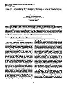
Figure 7.9. Rotation as three successive translations [76].

kernels in repetitive rotations experiments. In the rest of this chapter we will compare our optimized designs with the O-MOMS and B-splines, as functions belonging to the class of minimally supported PP basis functions. 7.3.4.1. The rotation experiment We have adopted the experiment with successive image rotations [76]. A test image is rotated to a certain angle which is the result of an integer division of 360◦ , for example, 24◦ = 360◦ /15, 36◦ = 360◦ /10, and so forth. The rotation is repeated until the image reaches its starting position. Consider the matrix ⎡

cos θ R(θ) = ⎣ sin θ

⎤ − sin θ ⎦

cos θ

(7.114)

.

It determines a rotation of the image coordinates (x, y) by the angle θ. The matrix factorization ⎡

cos θ R(θ) = ⎣ sin θ

⎤ − sin θ ⎦

cos θ

⎡

⎢1 =⎣

0

− tan

- .⎤ ⎡ θ 1 2 ⎥ ⎦·⎣

1

sin θ

⎤ ⎡

0⎦ ⎢1 ·⎣ 1 0

− tan

- .⎤

1

θ 2 ⎥ ⎦

(7.115)

decomposes the rotation into three 1D translations, as illustrated in Figure 7.9 [76]. Each subpixel translation is an interpolation operation with no rescaling. The repetitive rotation experiment is very appropriate for accumulating the interpolation errors, thereby emphasizing the interpolator’s performance [62]. Several well-known test images have been chosen because of their different frequency contents. Among them, the Barbara, mandrill, and patterns images that contain high-frequency and texture details, the geometrical image contains different radial frequencies, the Lena image is more like a low-frequency image, and the bridge contains some straight edges (Figure 7.10).

322


Figure 7.10. Test images with different frequency contents.

On the chosen set of images, we have performed 10 and 15 successive rotations of 36◦ and 24◦ , respectively, involving PP optimized interpolators, B-splines and O-MOMS of third and fifth degrees. As a measure of goodness, we have used the SNR between the initial image and the rotated one. Table 7.1 summarizes the results for the third-degree kernels, while Table 7.3 summarizes the results for the fifth-degree kernels. One can see that significant improvements are provided by some of the proposed modified B-splines for the relatively high-frequency image Barbara. Even improvements of more than 4 dB are achieved, compared to the classical fifth-degree B-spline and the O-MOMS. This argues the applicability of the chosen optimization technique, especially for high-frequency images. For relatively low-frequency images (like Lena), noticeable improvements can be achieved. We illustrate the improvement of interpolation quality by two visual examples. A portion of the Barbara image, namely, the high-frequency trousers (Figure 7.11) is shown after 15 × 24◦ rotations using three different PP interpolators of third degree. As can be seen in Figure 7.12 the most blurred image is the one obtained by the cubic B-spline. Our modified spline (3,1) gives the superior visual quality. To magnify the effect, the same images are enlarged by factor of two in Figure 7.13. The second example is the central part of the geometrical image (Figure 7.14) containing high radial frequencies. The images, resulting from 15 successive rotations of 24◦ and by using three interpolation kernels of third degree, are shown in Figure 7.15, whereas Figure 7.16 shows the same images enlarged by factor of two. Again, more details are preserved in the image rotated using the Mod B-spline (3,1).


323

Table 7.3. SNRs for optimized PP kernels of fifth degree in Table 7.2 after rotation 10 × 36◦ . Design no.

Bridge

Barbara

Geometrical

Lena

1

29.54

32.25

24.32

36.21

2

29.65

32.67

24.43

36.26

3

29.60

32.49

24.38

36.23

4

29.52

32.22

24.30

36.19

5

29.49

32.15

24.30

36.17

6

29.80

33.08

24.54

36.32

7

29.82

33.35

24.65

36.22

8

29.82

33.34

24.60

36.28

9

29.80

33.26

24.53

36.32

10

29.81

33.29

24.52

36.37

11

29.20

30.15

24.05

35.81

12

29.72

31.57

24.33

36.10

13

29.20

32.79

24.76

34.67

14

29.58

33.44

24.82

35.43

15

29.50

33.07

24.78

35.51

B-spline (5)

28.02

27.89

23.37

34.98

O-MOMS (5,3,1)

28.47

29.05

23.69

35.38

Figure 7.11. Portion of Barbara image: trousers (zoomed out).

Table 7.4 shows comparisons of different spline-based interpolations for four rotation experiments. Barbara image has been rotated clockwise 15 times by 24◦ and 10 times by 36◦ . The same successive rotations have been accomplished then backwards to allow for accumulating more interpolation errors. The differences between the original image and the rotated ones have been measured by peak signal-to-noise ratio (PSNR), signal-to-noise ratio (SNR), mean absolute error (MAE), mean square error, and maximum difference. The experiments have involved the interpolation kernels described in Section 7.3.4.2. The results in the

324


Figure 7.12. Results of successive rotations, 15 × 24◦ . From left to right: original image, rotated using cubic B-spline, rotated using O-MOMS (3,1), rotated using Mod B-spline (3,1).

Figure 7.13. Same as in Figure 7.11 magnified by a factor of two. From left to right and from top to bottom: original, cubic B-spline rotated, O-MOMS (3,1) rotated, Mod B-spline (3,1) rotated.

table once again confirm the superior performance of the properly optimized kernels. Note, that the modified B-spline kernel of third degree already achieves better performance than some of the higher degree kernels.


325

Figure 7.14. Portion of geometrical image: center (zoomed out).

Figure 7.15. Results of successive rotations, 15 × 24◦ . From left to right: original image, rotated using cubic B-spline, rotated using O-MOMS (3,1), rotated using Mod B-spline (3,1).

Figure 7.16. Same as in Figure 7.14 magnified by factor of two. From left to right and from top to bottom: original image, cubic B-spline rotated, O-MOMS (3,1) rotated, Mod B-spline (3,1) rotated.

7.3.4.2. Approximation error kernel The performance of different interpolators can be compared theoretically based on the representation of the approximation error (7.42), (7.54) in frequency domain [62]. We present a comparison between two modified B-spline-based optimized kernels, of third and fifth degrees, respectively, and their O-MOMS counterparts.

326


Table 7.4. Trend of some quality measures for different spline-based interpolators. Barbara (512×512) image processed.

Interpolator

Rotations 15 × 24◦ clockwise

PSNR,

SNR,

MAE

MSE

MaxDiff

[dB]

[dB]

L1 norm

L2 norm

L∞ norm

B-spline (3)

27.02

22.07

5.5717

0.0276

70

O-MOMS (3,1)

30.20

25.25

3.6765

0.0191

58

Mod B-spline (3,1)

32.64

27.70

2.9757

0.0144

50

B-spline (5)

31.19

26.25

3.3074

0.0171

50

O-MOMS (5,3,1)

32.41

27.89

2.8853

0.0148

46

Mod B-spline (5,3,1)

36.47

31.53

1.9769

0.0093

28

Rotations Interpolator

PSNR,

SNR,

[dB] B-spline (3) O-MOMS (3,1)

15 × 24◦

clockwise and back

MAE

MSE

MaxDiff

[dB]

L1 norm

L2 norm

L∞ norm

25.07

20.12

7.1015

0.0345

77

28.23

23.28

4.5958

0.0240

67

Mod B-spline (3,1)

30.40

25.46

3.9859

0.0019

60

B-spline (5)

28.98

24.04

4.2307

0.0220

60

O-MOMS (5,3,1)

30.21

25.27

3.6552

0.0191

55


34.14

29.20

2.5497

0.0121

34

Interpolator

Rotations 10 × 36◦ clockwise

PSNR,

SNR,

MAE

MSE

MaxDiff

[dB]

[dB]

L1 norm

L2 norm

L∞ norm

B-spline (3)

28.64

23.69

4.5812

0.0229

63

O-MOMS (3,1)

31.92

26.97

3.0177

0.0157

55

Mod B-spline (3,1)

34.03

29.08

2.5076

0.0123

49

B-spline (5)

32.92

27.97

2.7346

0.0140

49

O-MOMS (5,3,1)

34.11

29.16

2.4038

0.0122

44


37.89

32.95

1.7016

0.0079

26

Interpolator

PSNR,

SNR,

MAE

MSE

MaxDiff

[dB]

[dB]

L1 norm

L2 norm

L∞ norm

B-spline (3)

26.30

21.36

6.0891

0.0300

74

O-MOMS (3,1)

29.76

24.82

3.8270

0.0201

69

Mod B-spline (3,1)

31.65

26.71

3.3366

0.0162

72

B-spline (5)

30.51

25.56

3.5545

0.0185

59

O-MOMS (5,3,1)

31.77

26.83

3.0745

0.0160

56


35.81

30.87

2.1270

0.0100

31

Rotations 10 × 36◦ clockwise and back


327 0

−10

Magnitude (dB)

−20 −30 −40 −50 −60 −70 −80 −90

−100

0

0.5


2.5

3

B-spline (3) O-MOMS (3, 1) Mod (3, 1) Figure 7.17. Magnitude responses of three PP interpolators of third degree.

The O-MOMS interpolation kernels of the form (7.81) have been optimized to have minimal interpolation constant [9]. This has yielded interpolator functions of the type of (7.81) as follows: -

.

1 D2 β3 (x), 42 - . . 1 1 D2 β5 (x) + D4 β5 (x). βO-MOMS(5,3,1) (x) = β5 (x) + 33 7920 βO-MOMS(3,1) (x) = β3 (x) +

(7.116)

Here, the abbreviations O-MOMS(3, 1) and O-MOMS(5, 3, 1) denote the degrees of the B-splines involved in the combination. The modified kernels have been optimized to have a passband up to α = 0.35 with maximal ripples of 0.1–0.2% and to suppress the frequencies in the stopband as much as possible. The optimization has resulted in the kernels $

%

βmod(3,1) (x) = β3 (x) − 0.0714β1 (x) + 0.0357 β1 (x − 1) + β1 (x + 1) ,

βmod(5,3,1) (x) = β5 (x) − 0.1289β3 (x) + 0.0003β1 (x) $

+ 0.0678 β3 (x − 1) + β3 (x + 1) $

1

1

%

%

− 0.0022 β (x − 1) + β (x + 1) $ % − 0.0013 β1 (x − 2) + β1 (x + 2) .

(7.117)

Again, the notations Mod B-spline (3,1) and Mod B-spline (5,3,1) stand for the degrees of the B-splines involved in the corresponding combinations. Figure 7.17 compares the magnitude response of the optimized interpolation kernel of third degree (solid line), as of (7.90), with the O-MOMS (dashed line) and B-spline (dotted line) of same degree. It is well visible that the zeros of the

328

Interpolation by optimized spline kernels 0

Magnitude (dB)

−10 −20 −30 −40 −50 −60 −70 −80 −90

−100

0

0.5


2.5

3

B-spline (5) O-MOMS (5, 3, 1) Mod B-spline (5, 3, 1) Figure 7.18. Magnitude responses of three PP interpolators of fifth degree.

modified kernel are not all located at the multiples of the sampling rate. This results in a better stopband attenuation. The magnitude response of the fifth-degree modified B-spline interpolator (solid line), as of (7.94), is shown in Figure 7.18 together with O-MOMS (dashed line) and quintic B-spline (dotted line). Here, the effect of zero clustering for the case of modified B-spline interpolator is not indicated down to −100 dB. Much more can be seen from the curve of the error approximation kernel, as of (7.42). As can be seen in Figure 7.19, the O-MOMS kernels (dashed lines) perform better for low frequencies, while the modified B-spline kernels (solid lines) are superior for higher frequencies (the curves to the left are for the third-degree kernels and the curves to the right are for the fifth-degree kernels). Note, however, that for low frequencies the predictive approximation error in the case of modified B-splines is less than 10−6 ! This theoretical performance comparison concurs with the rotation experiment and shows that the modified kernels are potentially more promising because of their better high-frequency performance and reasonable and acceptable low-frequency error. 7.3.4.3. Total squared error The total squared approximation error can be predicted using (7.54) for different interpolators and for different image models [63]. We have computed the error (7.54) for the following image models: white noise, Markov process, and an edge (unit step function), involving the interpolators from Section 7.3.4.2. White noise. The power spectrum of the white noise is uniform and constant over the interval of integration. For this image model, the total squared error is obtained by integrating the error kernel (7.42) over the chosen interval. We


329

100

Error kernel

10−2 10−4 10−6 10−8 10−10

0.05 0.1 0.15 0.2 0.25 0.3 0.35 0.4 0.45 0.5 Normalized frequency B-spline (3) O-MOMS (3, 1) Mod B-spline (3, 1)

B-spline (5) O-MOMS (5, 3, 1) Mod B-spline (5, 3, 1)

Figure 7.19. Approximation error kernels for different PP interpolators.

Table 7.5. Predictive squared error for different image models and different interpolators. ε2 , [DB]

Interpolator

White noise

Markov process

B-spline (3) O-MOMS (3,1) Mod (3,1)

13.15 14.03 14.58

28.91 29.98 30.63

B-spline (5) O-MOMS (5,3,1)

14.94 15.47

31.02 31.62

Mod (5,3,1)

17.02

33.62

have adopted the settings in [63], namely, the integration interval has been set to [−π, π] (band-limited white noise). The results are summarized in Table 7.5. Markov process. The Markov process has been chosen as it models a large class of real images [63]. In frequency domain, its power spectrum is described by & & &Ga (2π f )&2 =

−2 log(ρ) (2π f )2 + log2 (ρ)

(7.118)

with a correlation factor ρ less than but close to unity. To be consistent with the experiments in [63], we have set ρ = 0.9. The results are presented in the last column of Table 7.5. Even for such a low-frequency process the modified interpolation kernels play better, a fact emphasizing once again the importance of a proper compromise in specifying the optimization criteria.

330


Edge (step function). The step function is a model of sharp changes in the image intensity, that is, image edges. It is not a band-limited function and the accuracy of its reconstruction by means of interpolation depends on the phase of the sampling process, that is, the relative position of the samples around the step. For this image model, the measure (7.42) gives the amount of the approximation errors averaged over all possible sampling phases. Assume an ideal rectangular scanning device aperture of unity length. It transforms the step function into the ramp function of unity width. Its spectrum is 2 & & &Ga (2π f )&2 = sinc (π f ) . 2

(2π f )

(7.119)

One can represent the averaged error as function of the sampling frequency. The curves for some traditional interpolators, such as sinc (the ideal interpolator for band-limited functions), linear, and piecewise cubic, have been obtained in [49]. We add here the curves for the cubic B-spline interpolator (Figure 7.20(a)) and for the optimized O-MOMS (3,1) and Mod (3,1) (Figure 7.20(b)). As can be seen from the figures, for such a nonband-limited model the sinc interpolator is outperformed by the spline-based interpolators for a large range of sampling ratios. Also, the frequency domain specified optimization criteria that lead only to marginal improvement in this particular case. 7.4. Conclusions In this section, we reviewed new spline-like basis functions, namely, PP functions of minimal support. We demonstrated how to improve the interpolation performance by taking optimized combinations of B-splines of different degrees. The combinations of third- and first-degree B-splines and of fifth-, third-, and firstdegree B-splines were especially studied because they provide a good opportunity to deal with both smooth and sharp image areas and because they offer acceptable computational complexity. Two optimization techniques were presented: first one based on approximation theoretic assumptions and second one operating in frequency domain just like in a classical filter design. By the latter technique, the adjusted parameters were optimized in such a way that the resulting interpolation function sufficiently suppresses the imaging frequencies. As a result, the obtained PP interpolation kernels achieved better frequency characteristics than the classical B-splines, that is, flatter in the passband, steeper in the transition band, and with sufficient attenuation in the stopbands. While being very similar in construction to the so-called O-MOMS functions, the main difference between two optimized families is in the position of frequency response zeros around the multiples of the sampling rate (2kπ in terms of angular frequency). MOMS functions have multiple zeros at those points complying with the Strang-Fix conditions for Lth-order approximation functions. In the alternative design, the Lth order of approximation is traded for a better frequency domain stopband performance. In fact, as a result of the minimax optimization procedure the obtained functions have zeros

331

Averaged approximation error


0.6

0.8

1 1.2 1.4 1.6 Sampling frequency

Sinc Linear Cubic

1.8

2

B-spline (3)

Averaged approximation error

(a)

0.6

0.8

1 1.2 1.4 1.6 Sampling frequency

1.8

2

B-spline (3) O-MOMS (3, 1) Mod B-spline (5, 3, 1) (b) Figure 7.20. Averaged approximation error for image model “edge scanned with ideal aperture” and for different interpolators.

clustered around (2kπ), thus forming the desired stopbands. We showed that this optimization technique, working entirely in frequency domain, gives very promising results. This is done thanks to the good compromise between the increased interpolation capabilities for relatively high frequencies and the controllable lowfrequency error. We experimentally proved the best interpolation capabilities of the functions thus constructed, especially for preserving high-frequency image details.

332


As far as the computational complexity is concerned, we described efficient filtering structures at arbitrary scale, based on the so-called Farrow structure. Thanks to their susceptibility to optimization and computationally efficient structures, the modified B-spline kernels can considerably increase the interpolation quality and, therefore, they can be applied in image rescaling and rotation tasks and in approximation of multiscale operators as well. Bibliography [1] A. Aldroubi and M. Unser, “Families of multiresolution and wavelet spaces with optimal properties,” Numerical Functional Analysis and Optimization, vol. 14, no. 5-6, pp. 417–446, 1993. [2] A. Aldroubi and M. Unser, “Families of wavelet transforms in connection with Shannon’s sampling theory and the Gabor transform,” in Wavelets: A Tutorial in Theory and Applications, C. K. Chui, Ed., vol. 2, pp. 509–528, Academic Press, Boston, Mass, USA, 1992. [3] A. Aldroubi and M. Unser, “Sampling procedures in function spaces and asymptotic equivalence with Shannon’s sampling theory,” Numerical Functional Analysis and Optimization, vol. 15, no. 12, pp. 1–21, 1994. [4] A. Aldroubi, M. Unser, and M. Eden, “Cardinal spline filters: stability and convergence to the ideal sinc interpolator,” Signal Processing, vol. 28, no. 2, pp. 127–138, 1992. [5] D. Babic, J. Vesma, T. Saramäki, and M. Renfors, “Implementation of the transposed Farrow structure,” in Proceedings of IEEE International Symposium on Circuits and Systems (ISCAS ’02), vol. 4, pp. 5–8, Phoenix, Ariz, USA, May 2002. [6] G. Battle, “A block spin construction of ondelettes. I. Lemarié functions,” Communications in Mathematical Physics, vol. 110, no. 4, pp. 601–615, 1987. ˚ Björck, Numerical Methods for Least Squares Problems, SIAM, Philadelphia, Pa, USA, 1996. [7] A. [8] T. Blu, P. Thévenaz, and M. Unser, “Minimum support interpolators with optimum approximation properties,” in Proceedings of International Conference on Image Processing (ICIP ’98), vol. 3, pp. 242–245, Chicago, Ill, USA, October 1998. [9] T. Blu, P. Thévenaz, and M. Unser, “MOMS: maximal-order interpolation of minimal support,” IEEE Transactions on Image Processing, vol. 10, no. 7, pp. 1069–1080, 2001. [10] T. Blu and M. Unser, “Quantitative Fourier analysis of approximation techniques. I. Interpolators and projectors,” IEEE Transactions on Signal Processing, vol. 47, no. 10, pp. 2783–2795, 1999. [11] C. de Boor, A Practical Guide to Splines, Springer, New York, NY, USA, 2nd edition, 2001. [12] C. de Boor, R. A. DeVore, and A. Ron, “Approximation from shift-invariant subspaces of L2 (Rd ),” Transactions of the American Mathematical Society, vol. 341, no. 2, pp. 787–806, 1994. [13] P. J. Burt, “Fast filter transform for image processing,” Computer Graphics and Image Processing, vol. 16, no. 1, pp. 20–51, 1981. [14] S. Chaudhuri, Ed., Super-Resolution Imaging, Kluwer Academic, Boston, Mass, USA, 2001. [15] C. K. Chui, Multivariate Splines, vol. 54 of CBMS-NSF Regional Conference Series in Applied Mathematics, SIAM, Philadelphia, Pa, USA, 1988. [16] C. K. Chui and J.-Z. Wang, “On compactly supported spline wavelets and a duality principle,” Transactions of the American Mathematical Society, vol. 330, no. 2, pp. 903–915, 1992. [17] A. Cohen, I. Daubechies, and J.-C. Feauveau, “Biorthogonal bases of compactly supported wavelets,” Communications on Pure and Applied Mathematics, vol. 45, no. 5, pp. 485–560, 1992. [18] K. Egiazarian, T. Saramäki, H. Chugurian, and J. Astola, “Modified B-spline filters and interpolators,” in Proceedings of IEEE International Conference on Acoustics, Speech, Signal Processing (ICASSP ’96), vol. 3, pp. 1743–1746, Atlanta, Ga, USA, May 1996. [19] C. Farrow, “A continuously variable digital delay element,” in Proceedings of IEEE International Symposium on Circuits and Systems (ISCAS ’88), pp. 2641–2645, Espoo, Finland, June 1988. [20] F. W. Gembicki, Vector optimization for control with performance and parameter sensitivity indices, Ph.D. thesis, Case Western Reserve University, Cleveland, Ohio, USA, 1974.


333

[21] A. Gotchev, J. Vesma, T. Saramäki, and K. Egiazarian, “Digital image resampling by modified Bspline functions,” in Proceedings of IEEE Nordic Signal Processing Symposium (NORSIG ’00), pp. 259–262, Kolmarden, Sweden, June 2000. [22] A. Gotchev, J. Vesma, T. Saramäki, and K. Egiazarian, “Multiscale image representations based on modified B-splines,” in Proceedings of International Workshop on Spectral Techniques and Logic Design (SPEGLOG ’00), pp. 431–452, Tampere, Finland, June 2000. [23] A. Gotchev, K. Egiazarian, J. Vesma, and T. Saramäki, “Edge-preserving image resizing using modified B-splines,” in Proceedings of IEEE International Conference on Acoustic, Speech and Signal Processing (ICASSP ’01), vol. 3, pp. 1865–1868, Salt Lake City,Utah, USA, May 2001. [24] A. Gotchev, K. Egiazarian, and T. Saramäki, “Comparing the performance of optimized piecewise polynomial image interpolators,” in Proceedings of IEEE Nordic Signal Processing Symposium (NORSIG ’02), Hurtigruta, Norway, October 2002, CDROM Proceedings SatAmOr4. [25] A. Gotchev, T. Saramäki, and K. Egiazarian, “Spline and Wavelet Based Techniques for Signal and Image Processing,” doctoral thesis, Tampere University of Technology, Tampere, Finland, September 2003. [26] A. Gotchev and K. Egiazarian, “Spline-based resampling of noisy images,” in Proceedings of the 2nd International Symposium on Image and Signal Processing and Analysis (ISPA ’01), pp. 580– 585, Pula, Croatia, June 2001. [27] A. Gotchev, G. Marchokov, T. Saramäki, and K. Egiazarian, “Efficient algorithms and structures for image size reduction,” in Proceedings of TICSP International Workshop on Spectral Methods and Multirate Signal Processing (SMMSP ’02), pp. 251–258, Toulouse, France, September 2002. [28] A. Gotchev, K. Egiazarian, G. Marchokov, and T. Saramäki, “A near least squares method for image decimation,” in Proceedings of International Conference on Image Processing (ICIP ’03), vol. 3, pp. 929–932, Barcelona, Spain, September 2003. [29] T. Hentschel and G. Fettweis, “Continuous-time digital filters for sample-rate conversion in reconfigurable radio terminals,” in Proceedings of the European Wireless Conference (EW ’00), pp. 55–59, Dresden, Germany, September 2000. [30] H. S. Hou and H. C. Andrews, “Cubic splines for image interpolation and digital filtering,” IEEE Transactions on Acoustics, Speech, and Signal Processing, vol. 26, no. 6, pp. 508–517, 1978. [31] R. Hummel, “Sampling for spline reconstruction,” SIAM Journal on Applied Mathematics, vol. 43, no. 2, pp. 278–288, 1983. [32] A. Jain, Fundamentals of Digital Image Processing, Prentice-Hall, Englewood Cliffs, NJ, USA, 1989. [33] R. G. Keys, “Cubic convolution interpolation for digital image processing,” IEEE Transactions on Acoustics, Speech, and Signal Processing, vol. 29, no. 6, pp. 1153–1160, 1981. [34] R. Lagendijk and J. Biemond, Iterative Identification and Restoration of Images, Kluwer Academic, Boston, Mass, USA, 1991. [35] T. M. Lehmann, C. Gonner, and K. Spitzer, “Survey: interpolation methods in medical image processing,” IEEE Transactions on Medical Imaging, vol. 18, no. 11, pp. 1049–1075, 1999. [36] P. Lemarié, “Ondelettes a` localisation exponentielle,” Journal de Mathématiques Pures et Appliquées, vol. 67, no. 3, pp. 227–236, 1988. [37] S. G. Mallat, “A theory for multiresolution signal decomposition: the wavelet representation,” IEEE Transactions on Pattern Analysis and Machine Intelligence, vol. 11, no. 7, pp. 674–693, 1989. [38] S. Mallat, A Wavelet Tour of Signal Processing, Academic Press, San Diego, Calif, USA, 1998. [39] G. Marchokov, A. Gotchev, J. Vesma, T. Saramäki, and K. Egiazarian, “Efficient polynomial-based methods for image resizing,” in Proceedings of the 3rd International Conference on Information, communications, and Signal Processing (ICICS ’01), p. 5, Singapore, October 2001, CD-ROM Processing, 2D1.3. [40] E. H. W. Meijering, K. J. Zuiderveld, and M. A. Viergever, “Image reconstruction by convolution with symmetrical piecewise nth-order polynomial kernels,” IEEE Transactions on Image Processing, vol. 8, no. 2, pp. 192–201, 1999.

334


[41] E. H. W. Meijering, W. J. Niessen, and M. A. Viergever, “Quantitative evaluation of convolutionbased methods for medical image interpolation,” Medical Image Analysis, vol. 5, no. 2, pp. 111– 126, 2001. [42] A. Mertins, Signal Analysis, John Wiley & Sons, New York, NY, USA, 1999. [43] S. Mitra, Digital Signal Processing: A Computer-Based Approach, McGraw-Hill, New York, NY, USA, 2001. [44] A. Muñoz, T. Blu, and M. Unser, “Least-squares image resizing using finite differences,” IEEE Transactions on Image Processing, vol. 10, no. 9, pp. 1365–1378, 2001. [45] N. Nguyen, P. Milanfar, and G. Golub, “A computationally efficient superresolution image reconstruction algorithm,” IEEE Transactions on Image Processing, vol. 10, no. 4, pp. 573–583, 2001. [46] A. Oppenheim and R. Shafer, Discrete-Time Signal Processing, Prentice-Hall, Englewood Cliffs, NJ, USA, 1989. [47] Optimization Toolbox User’s Guide, MathWorks, 2002. [48] S. K. Park and R. A. Schowengerdt, “Image sampling, reconstruction, and the effect of samplescene phasing,” Applied Optics, vol. 21, no. 17, pp. 3142–3151, 1982. [49] S. K. Park and R. A. Schowengerdt, “Image reconstruction by parametric cubic convolution,” Computer Vision, Graphics, and Image Processing, vol. 23, no. 3, pp. 258–272, 1983. [50] S. Pissanetzky, Sparse Matrix Technology, Academic Press, London, UK, 1984. [51] G. Ritter and J. Wilson, Handbook of Computer Vision Algorithms in Image Algebra, CRC Press, Boca Raton, Fla, USA, 2000. [52] B. Romeny, Ed., Geometry-Driven Diffusion in Computer Vision, Kluwer Academic, Dordrecht, The Netherlands, 1994. [53] A. Ron, “Factorization theorems for univariate splines on regular grids,” Israel Journal of Mathematics, vol. 70, no. 1, pp. 48–68, 1990. [54] J. Russ, The Image Processing Handbook, CRC Press, Boca Raton, Fla, USA, 2002. [55] T. Saramäki, “Finite impulse response filter design,” in Handbook for Digital Signal Processing, S. Mitra and J. Kaiser, Eds., pp. 155–277, John Wiley & Sons, New York, NY, USA, 1993. [56] A. Schaum, “Theory and design of local interpolators,” CVGIP: Graphical Models and Image Processing, vol. 55, no. 6, pp. 464–481, 1993. [57] C. E. Shannon, “Communication in the presence of noise,” Proceedings of IEEE, vol. 86, no. 2, pp. 447–457, 1998. [58] I. Schoenberg, Cardinal Spline Interpolation, SIAM, Philadelphia, Pa, USA, 1973. [59] G. Strang and G. Fix, “A Fourier analysis of the finite-element variational method,” in Constructive Aspect of Functional Analysis, pp. 796–830, Edizioni Cremonese, Rome, Italy, 1971. [60] G. Strang and T. Nguyen, Wavelets and Filter Banks, Wellesley-Cambridge Press, Wellesley, Mass, USA, 1996. [61] P. Thévenaz, T. Blu, and M. Unser, “Complete parameterization of piecewise polynomial interpolators according to degree, support, regularity, and order,” in Proceedings of International Conference on Image Processing (ICIP ’00), vol. 2, pp. 335–338, Vancouver, BC, Canada, September 2000. [62] P. Thévenaz, T. Blu, and M. Unser, “Image interpolation and resampling,” in Handbook of Medical Imaging, Processing and Analysis, I. N. Bankman, Ed., pp. 393–420, Academic Press, San Diego Calif, USA, 2000. [63] P. Thévenaz, T. Blu, and M. Unser, “Interpolation revisited,” IEEE Transactions on Medical Imaging, vol. 19, no. 7, pp. 739–758, 2000. [64] M. Unser, “Approximation power of biorthogonal wavelet expansions,” IEEE Transactions on Signal Processing, vol. 44, no. 3, pp. 519–527, 1996. [65] M. Unser, A. Aldroubi, and M. Eden, “Fast B-spline transform for continuous image representation and interpolation,” IEEE Transactions on Pattern Analysis and Machine Intelligence, vol. 13, no. 3, pp. 277–285, 1991. [66] M. Unser and A. Aldroubi, “A general sampling theory for non-ideal acquisition devices,” IEEE Transactions on Signal Processing, vol. 42, no. 11, pp. 2915–2925, 1994.


335

[67] M. Unser, A. Aldroubi, and M. Eden, “Polynomial spline signal approximations: filter design and asymptotic equivalence with Shannon’s sampling theorem,” IEEE Transactions on Information Theory, vol. 38, no. 1, pp. 95–103, 1992. [68] M. Unser, A. Aldroubi, and M. Eden, “On the asymptotic convergence of B-spline wavelets to Gabor functions,” IEEE Transactions on Information Theory, vol. 38, no. 2, part 2, pp. 864–872, 1992. [69] M. Unser, A. Aldroubi, and M. Eden, “B-spline signal processing. I. Theory,” IEEE Transactions on Signal Processing, vol. 41, no. 2, pp. 821–833, 1993. [70] M. Unser, A. Aldroubi, and M. Eden, “B-spline signal processing. II. Efficient design and applications,” IEEE Transactions on Signal Processing, vol. 41, no. 2, pp. 834–848, 1993. [71] M. Unser, A. Aldroubi, and M. Eden, “A family of polynomial spline wavelet transforms,” Signal Processing, vol. 30, no. 2, pp. 141–162, 1993. [72] M. Unser, A. Aldroubi, and S. J. Schiff, “Fast implementation of continuous wavelet transforms with integer scale,” IEEE Transactions on Signal Processing, vol. 42, no. 12, pp. 3519–3523, 1994. [73] M. Unser, “Splines: a perfect fit for signal and image processing,” Signal Processing Magazine, vol. 16, no. 6, pp. 22–38, 1999. [74] M. Unser and T. Blu, “Wavelet theory demystified,” IEEE Transactions on Signal Processing, vol. 51, no. 2, pp. 470–483, 2003. [75] M. Unser and I. Daubechies, “On the approximation power of convolution-based least squares versus interpolation,” IEEE Transactions on Signal Processing, vol. 45, no. 7, pp. 1697–1711, 1997. [76] M. Unser, P. Thévenaz, and L. P. Yaroslavsky, “Convolution-based interpolation for fast, highquality rotation of images,” IEEE Transactions on Signal Processing, vol. 4, no. 10, pp. 1371–1381, 1995. [77] J. Vesma and T. Saramäki, “Polynomial-based interpolation filters—part I: filter synthesis,” to appear in Circuits, Systems and Signal Processing, vol. 26, no. 1, 2007. [78] M. Veterli and H. Kovacevic, Wavelets and Subband Coding, Prentice-Hall, New York, NY, USA, 1995. [79] G. Wahba, “Practical approximate solutions to linear operator equations when the data are noisy,” SIAM Journal on Numerical Analysis, vol. 14, no. 4, pp. 651–667, 1977. [80] Y.-P. Wang and S. L. Lee, “Scale-space derived from B-splines,” IEEE Transactions on Pattern Analysis and Machine Intelligence, vol. 20, no. 10, pp. 1040–1055, 1998. [81] A. P. Witkin, “Scale-space filtering,” in Proceedings of the 8th International Joint Conference on Artificial Intelligence (IJCAI ’83), pp. 1019–1022, Karlsruhe, Germany, August 1983. [82] L. P. Yaroslavsky and M. Eden, Fundamentals of Digital Optics, Birkhäuser, Boston, Mass, USA, 1996. [83] L. P. Yaroslavsky, “Fast signal sinc-interpolation methods for signal and image resampling,” in Image Processing: Algorithms and Systems, vol. 4667 of Proceedings of SPIE, pp. 120–129, San Jose, Calif, USA, January 2002.

Atanas Gotchev: Institute of Signal Processing, Tampere University of Technology, P.O. Box 553, 33101 Tampere, Finland Email: [email protected] Karen Egiazarian: Institute of Signal Processing, Tampere University of Technology, P.O. Box 553, 33101 Tampere, Finland Email: [email protected] Tapio Saramäki: Institute of Signal Processing, Tampere University of Technology, P.O. Box 553, 33101 Tampere, Finland Email: [email protected]