Copyright 0 1995 by the Genetics Society of America
Interval Mapping of Quantitative Trait Loci Employing Correlated Trait Complexes Abraham B. Korol, Yefim I. Ronin and Valery M. Kirzhner Institute of Evolution, University of Haifa, Haifa 31 905, Israel
Manuscript received September 6, 1994 Accepted for publication April 11, 1995 ABSTRACT An approach to increase the resolution power of interval mapping of quantitative trait (QT) loci is proposed, basedonanalysisof correlated trait complexes. For a given set of QTs, the broad sense heritability attributed toa QT locus (QTL) (say, A / a ) is an increasing functionof the number of traits. Thus, for some traits x and y, H $ ( A / a ) 2 HH ( A / a ) . The last inequality holds even if y does not depend on A / a at all, but x and y are correlated within the groups AA, Aa and aa due to nongenetic factors and segregationof genes from other chromosomes.A simple relationship connects H' (both in single trait and two-trait analysis) with the expected LOD value, ELOD = -'/nN log( 1 - H ' ) . Thus, situations could exist that from the inequality H $ ( A / a ) 2 HH ( A / a ) a higher resolution is provided by the two-trait analysis as compared to the single-trait analysis, in spite of the increased number of parameters.Employing LOD-scoreprocedure to simulated backcross data, we showed that the resolution power of the QTL mapping model can be elevated if correlation between QTs is taken into account. The method allows us to test numerous biologically important hypotheses concerning manifold effects of genomic segments on the defined trait complex (means, variances and correlations).
T
HE resolution of marker analysisof quantitative
trait variation is a major factor affecting practical applications of quantitative trait locus (QTL) mapping. A detailed discussion of the issues concerningthe power of tests for detecting linkage can be found in and GENIZI1978; DEmany publications (e.g., SOLLER MENAIS et al. 1988; LANDER and BOTSTEIN1989; SOLLER 1990; WELLERand WYLER 1992; CARBOand BECKMANN NELL et al. 1993). The precision of the parameter estimation depends on the effect of the QT locus in question relative to the total phenotypic variance of the trait in the mapping population. In otherwords, the higher the discrepancy between the distribution densities of x) for a backthe QT locus groups [fu( x ) and ha( cross], the better is the expected resolution. Several procedures have been proposed to improve the precision of mapping, including the multimarker (interval mapping) analysis (LANDER and BOTSTEIN1989;KNOTT and HALEY 1992), selective sampling ( LEBOWITZ et al., 1987; CAREY and WILLIAMSON 1991; DARVASI and and SOLLER 1992), replicated progeny testing ( SOLLER BECKMANN1990),and sequential experimentation ( BOEHNKE and MOLL 1989; MOTRO and SOLLER 1993) . Recently, much attention has been paid to improve the efficiency of marker analysis of QTL by taking into accountthedependence of the quantitative trait on many QT loci (genomic segments) (JANSEN and STAM 1994; ZENC 1994). A situation when one QT locus (or Corresponding author: A. B. Korol, Institute of Evolution, University of Haifa, Mount Camel, Haifa 31905, Israel. E-mail:
[email protected] C:enetics 140: 1137-1147 (July, 1995)
a chromosome segment defined by a pair of flanking markers) affects simultaneously several QTs could also be considered. Such analysis may be of major importance in formulating marker-assisted breeding strategies, d i s secting heterosis as a multilocus multitrait phenomenon, developing optimized programs for evaluation and b i e conservation of genetic resources, revealing genetic architecture of fitness systems in natural populations, etc. Multivariate approach in segregation and linkage analysis of quantitative traits was recently used in human genetics (e.g.,AMES and LAINC 1993) but has not yet been applied for QTL mapping. In mapping QTloci, the experimental design usually includes simultaneous measurements of many QTsand subsequent treatment of these individual traits. Results obtained in many recent studies showed that some genomic segments indeed affect several traits (e.g., EDWARDS et al. 1992; DOEBLEYand STEC 1993) . Multimaker analysis allows multiple effects of any segment being estimated, if measurements of many traits are available. Nevertheless, in many current QTL mapping methods eachtrait is analyzed separately (but SeeJIANG and ZENG 1995).As will be shown in this paper, a substantial amount of genetic transmission information available in the data may be lost by this approach. Consequently, an increase in resolution power of QTLmarker linkage analysis can be achieved by accounting of correlations between the QTs, i.e., when one considers joint distributions of several traits in the QT locus groups [faa ( x, y ) a n d h a( x, y ) rather than themarginal distributions faa ( x) and fAu ( x ) , or A',, ( y ) and f A d ( y ) 1 . Earlier we showed the increased efficiencyof the
A. B. Korol, Y. I. Ronin and V. M. Kirzhner
1138
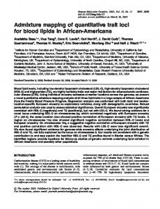
FIGURE1.-Joint distribution f ( x , y ) of two correlated traits, x and y, in backcross population. Even with the clearcut bimodality o f f ( x , y ) [when the components f a ( x , y ) and f A n ( x , y ) are far enough and thecorrelation is high] the marginal distributionsf( x ) a n d f ( y ) are unimodal. ( A ) The QT locus affects both traits, x and y. ( B ) The QTlocus affects only one of the traits, x.
multitrait analysis for differentprogeny types in estimating linkage between a QT locus and a single marker locus ( KOROL et al. 1987, 1994; RONINet al. 1995). The objectiveof this paper is to demonstrate the advantages of the multitrait analysis within the framework of interval mapping of QTL (see also JIANG and ZENG 1995). Besides of increased power of the statistical test and higher precision of estimation of the genetic parameters, the proposed approach allows for an integral evaluation of the effects of genomic segments on defined trait complexes (mean values, variancesand covariances). Because of the internal balance of the organism's systems ( SCHMALHAUSEN 1942),such an approach for QTL mapping seems to be much more justified biologically than the usual trait-by-trait analysis. GENERAL DESCRIPTION OF THE METHOD
The model: Consider a genomic segment carrying a QT locus (with alleles A and a) that affects two quantitative traits, xand y. We will confine ouranalysis to thebackcross situation. Any other type of mapping population may be treated in a similar way. In theillustration presented in Figure 1, the marginal densities are strongly overlapped. Without accounting of any additional information, based only on the observed marginal distributions f( x ) and f ( y ) , one would hardly assume that the progeny is polymorphic for an oligogene ( A / a). Nevertheless, the presence of an oligogene can easily be seen from the jointdistribution f ( x , y ) . In general, one may assume that the putative QT locus affects not only the mean values of the traits but also the trait variances and covariance. In such a case, the two-dimensional phenotype ( x , y ) of an arbitrary individual of a backcross progeny can be modeled as follows: x = m, + 0.5 d,g
+ e,,
y
= my
+ 0.54g + e,.
x and y are the individual's phenotype scores of the analyzed QTs, m, and m, are trait means, d, and 4 are the effects of substitution aa --t Aa with respect to mean values of x and y (i.e., d, = pxAa - px,, and 4 = pyAI, - pya), g denotes the genotype at locus A / a ( g = - 1 for aa and 1 for A a ) , e, is a random variable with zero mean and variances a:, and a& for g = -1 and g = 1; similarly, er is a random variable with mean zero and variances a:? and a:?.The variables e, and er are assumed to be correlated with correlation coefficients Rlq and &q for g = -1 and g = 1, respectively. Correlation between the traits x and y within the QT locus groups may be
due to other segregating QTLs or nongenetic correlation. Although we may assume that locus A / a can also affect trait variances and covariance, in this paper however we will deal mainly with the situation of equal variance-covariance matrix, 2, in the groups aa and Aa, i e . , 2,= X' = 2. In one trait analysis, the power and precision of QTL mapping analysis dependontheproportion of the variance caused by segregation of the putative QTL in the total variance of the trait x in the population, H : . Indeed, the expected LOD value for a backcross when the position of the closest marker coincides with that of the QTL is (see LANDER and BOTSTEIN1989)
where gfxpis the trait variance associated with the putative QTL ( uexp= d') and aKris the residual variance, so that H: = o:xp/ ( asx, + a$.).As shown in APPENDIX A the same relationship holds for the bivariate case, with a properly defined H:, a two-dimensional analogue of H : ,
where
-
[R,
+ d,4/(4aflY)
J2.
The parameter H $ obtained in APPENDIX A coincides with a natural bivariate analogue of H : based on the standard multivariate generalization of variance as a measure of variability. Namely, in measuring variability, determinant of the variance-covariance matrix, I Z 1 , is considered as such a generalization ( SOKAL1965) . If so, then one may formulate the multivariate (e.g., bivariate) analogue of H : as the proportion of the determinant of the variance-covariance matrix = CAa= X ) , caused by segregation of A / a (assuming relative to that of the variance-covariance matrix of the total fined in this way coincides with H$ from ( 3 ) derived from the ELOD (see APPENDIX A ) . Due to ( 2 ) , one could expect the resolution power of the analysis increases as H i , does. Clearly, statistical aspects concerned with possible increase in the number of parameters to be estimatedand changesin the degrees of freedom should be taken into account. Given fixed d x / a x , or HZ = '/,dp / ( '/*d: + a:),how could we increase the resolution by taking into account other traits? Clearly, if R, = 0, the effect of an additional trait is simply due to the increased euclidian distance between the (two-dimensional) centers of the groups aa and A / a. It is easy to see from ( 3 ) , that if dr f 0, & f 0 and sign ( G , d x 4 )< 0, then H $ 2 H: and one could expect a respective increase in resolution. Moreover, the inequality H $ > H ; holds even if &, = 0, but & f 0, no matter what sign of correlation we have. It iseasy to show (APPENDIX B ) that ( 3 ) is invariant with respect to nondegenerate linear transformation of the variables. Consequently, one may assume that mappingproblems with the same level of H i , could be considered as formally equivalent with the only complication due to the possibility of different number of the degrees of freedom. For instance, it may be of interest to compare equivalent (i.e., with the same value of H $ , while withdifferent values of other parameters) situations: (1, f 0, d, f 0 and R,f 0 (locus A / a affects two correlated traits) ; d, # 0 , 4 = 0 and R, f 0 (locus A / a affects x but not y, while within each of the groups Aa and aa the traits x and y are correlated); d, f 0, 4 f 0 and R, = 0 (locus A / a affects two noncorrelated traits) etc. The proximity of different situations with the same level of H ;
1139
Interval Analysis Multitrait QTL will be demonstrated on differentexamples both for the power of the log-likelihood ratio test and for theprecision of parameter estimation. Mixture-modelformulation for multitrait interval analysis: Interval mapping of QTL based on multitrait analysis can be conductedemploying the same techniques that were developed for the single-trait analysis (e.g., LANDER and BOTSTEIN 1989; JANSENS and STAM1994). The only difference is the increased number of parameters to be estimated and tested. Our pilot analysis with available experimental data on sweet corn (Y. TADMOR, Y. RONIN,A. KOROL,A. BAR-ZUR, and E. NEVO,unpublished results) shows that in many situations improved resolution makes up the latter drawback. Assume that a QT locus A / a resides insome interval flanked by two marker loci, MI/ ml and M2/ m,with recombination rates rl and r2 in intervals M l / m l - A / a and A / a - M 2 / T . Different modes of exchange interference in the interval could be considered; we will confine ourselves to the no interference case, so that r = rl z2 - 2rlr2, where r is the rateof recombination between MI/ ml and M2/ m. Based on the markerscores and themeasurements of traits of interest ( x and y ) for individuals from the mapping population, we should test whether or notvariation of x and/or y indeed depends on theinterval MI/ ml - M2/ m, and, if yes, identify the corresponding locus A / a . For a backcross case, the expected joint distributions of the traits x and y in each of the marker groups, Umlrn' ( x , y ) = UI ( x , y ) , U , l m 2( x , y ) = U, (x, y ) , L S ~ I M Z ( X , Y )= G ( x , y ) a n d U,I.MZ(X,Y) = &(X,y),can be written as follows:
+
the proportions 7 r t = T , ( rl , r 2 ) being dependent of the unknown recombination rates rl and rz. With no interference, 7 r l = (1 - rl) ( 1 - a ) / ( l - r),7r2 = rl (1 - r z ) / r , 7 r 3= 1 - 7 r 2 , and x4 = 1 - 7 r l . The specification of the densities A'.( x, y ) and ha(x, y ) depends on the assumptions made about the genetic control of the traits. Thus, if one assumes that no other oligogenes affecting x and/ ory are segregating, then two-dimensional normal density could be a good approximation, &,(X,
y)
=
[ 2 ~ 0 ~ -~R')]"'' ( 1
x exp{
-
xexp{-
2(1
1 -
R')[
( x - bxl)2
u:
2(1 1 R')[ ( x -0: PL30L)2
here px, and pyt ( i = 1, 2 ) are the expected mean values of x and y in groups aa ( i = 1 ) and Aa ( i = 2 ) , u x ,uyand R are the standarddeviations and correlation between x and y. The assumption of normality could also be suitable if several QTLs affecting the traits in question are segregating independently of A / a. To take into account possible deviations from normality caused by a strong gene on another chromosome we can represent each of the densities, fna ( x, y ) and f A a ( x, y ) as a sum of two bivariate normals (see also KNOTT and HALEV 1992). LOD-score test and parameter estimation: Assuming that
locus A / a is situated in the interval MI / ml - M 2 / nq!, the log-likelihood for a sampleof two-dimensional measurements xh, y k in marker groups with sizes N, ( i = 1, 4 ) can be written as N*
4
In L(8nl) =
C C In U ( x k , ,=I
k=l
4
Nt
In
=
yk)
[rrfaa(Xk, Y k )
+ ( l - 7 r z ) f A n ( X k , yk)].
t=1 k = l
In the general case of d, f 0 , d, f 0, and X,,, f X A a , so that Q n l = { T I , p x l , p x ~ pyl, , pp, u x l ,u x 2 uylr , uy2,R l , R21 is the vector of n1 = 11 unknown parameters, specifymg recombination rate and joint distributions of traits x and y in the QTL groups aa and Aa (in case of F2, Q n l could include up to 16 parameters). The assumption of no effect of genes from the interval MI/ ml - M 2 / q on the traits ( x , y ) can formally be presented by another set of parameters, Q = On, = { p x , py, ox,u y ,R) (the null hypothesis { H,: 0 = Q n o ) as contrasted to the alternative one {HI: 8 = /In1 1). According to thelikelihood ratio test approach (WILKS1962), if H , is true, the statistics
2 ln[max L ( Q , , ) /max L ( Q n O ) ] (5) 8 n 1 E SI Qno E $1 is distributed asymptotically as chi squarewith nl - no degrees X'
=
of freedom, where & and SI are the parameter spaces corresponding to Ho and H I , respectively (WILKS1962). Thus, if X' exceeds somecritical value, corresponding to a presetlevel of significance a , the null hypothesis can be rejected. In such a case, the numerical values providing maximum to L ( Bnl ) could be considered as maximum likelihood estimates of the parameters characterizing our QT locus A / a ( K N O and ~ HALEY 1992). However, in the multi-interval mapping the problem of the exact asymptotic distribution of the test statistics remains unsolved even in the single trait analysis (see ZENC 1994). If so, one could use extensive Monte-Carlo simulations to obtain anempirical critical value of the statistics for each considered situation. Two additional points are worth mentioning here. Introduction of any (additional) parameter( s ) specifylng the QTL mapping model should be justifiedstatisticallyby comparison to the corresponding reduced model. This is relevant to any complication of the QTL mapping model including the replacementof single-trait mapping analysis by its multitrait analogue. Thus, if one starts with the full formulation of HI : {Q = Q,,l, nl = 11) specifylng the putative QTL, then consequently reduced versions of HI should be tested, e.g., those with X,, = XAo ( Bnl = { rl , pxl, p % , pyl, py2,ox,cry, R ) , n l = 8 ) , etc. Parameters that d o not affect the significance level should be removed from the mapping model. An increase in the number of parameters in the two-trait mapping model does not necessary mean a substantial increase in the number of degrees of freedom of the test statistics. That is because the number of parameters specifymg the null hypothesis Ho = ( n o QTL in the considered interval) also increases. SIMULATIONPROCEDURE AND OPTIMIZATION
Generating the data: Monte-Carlo simulations were used to produce the observations. For each situation studied, 200 repeated mapping populations have been generated using pseudorandomnumbers. Bivariate normal distribution was used for the trait groups aa and Aa. However, our numerical results show (see be-
1140
A. B. Korol, Y . I. and Ronin
V. M. Kirzhner
low) that bivariate QTL mapping analysis is rather rowhere the highest value ofthe test statistics was achieved bust with respect to deviation from normality assumpin the proper interval (not in the neighboring ones). tion caused by independent segregation of other QTLs. Estimating the accuracy of obtained solutions: Usually, variances or SE of the estimates are employed as a For comparative analysis ofdifferent methodsand situameans foraccuracy comparison of the estimation procetions we used the same set of data. The composition of dures. However, in addition to random fluctuations the marker groups (mixtures U,, i = 1, 4 ) were modaround the mean, another possible source of distureled as binomial distributions with expected proporbances, the bias of the estimates, should also be taken tions 7 r t ( q , 3) and 1 - 7 r t ( q , r 2 ) . For most of the intoaccount.Thus, one should simultaneously take experiments,parameter values used for simulations care of the estimation variance and estimate bias. Morewere in the following range: 0 5 d, = xArr - x,, 5 0.6, over, each of these two components of the deviation of 0 5 dy = y A n - yrLn5 0.6, uno= 1, uAn = 1, 0 5 1 RI 5 the estimates from the true value could depend on the 0.7, N = 250. The length of the marker interval 20 cM level of the parameters. To allow for possible differwith the QT locus in the middle. No interference was assumed in the data presented below (and HALDANE'S ences in biases of the estimates, we employed the absolute error of the estimate, averaged over the repeated mapping functionis suitable) , but this restriction is not experiments: essential and the proposed method of analysis can be conducted with any other modeof multiple exchanges. 1 " 6u = - uJ, Obtaining numericalsolutions: The target of this k=l workwas to compare the above described approach with the single trait analysis, or to put it more exactly, where & and u are, respectively, the estimated and expected values of the parameter u ( i.e., u can be any comto estimate the gain in accuracy when the correlation ponent of the vector 8, say q , p x l , d,, pyl, 4 , u:, etc). between the quantitative traits is taken into account. Therefore, we do not dwell enough in this study on problems of numerical procedures of multi-extrema1 SIMULATION RESULTS multidimensional optimization. The main objective For the backcross case, we have simulated and anahere was to check how thecorrelation between the lyzed a number of situations when a QT locus ( A / a ) considered traits affects the detection power of the likeresiding in a markerinterval (MI/ ml - M 2 / m ) affects lihood ratio test and closeness of the optimal points simultaneously two correlated QTs, x and y. To show (representing the estimate of the parameter vector H ) the advantages of the proposed approach, we compare to the true parameter set. For this specific goal, we do the resulting characteristics (test power and precision not have to search the solution starting from arbitrary of the estimates) with those obtained using single-trait points. The simplest way to obtain the necessary estianalysis as well as two-trait analysis with no correlation mates is to use as an initial point in the optimization between the QTs. Two versions of Ho ( n o QTL in the procedure the parameter values equal to the true ones interval in question) will be considered: no other QTL of theconsidered sample (e.g., TITTERINGTON et al. in the genome, so that the normal distribution could 1985). Based on numerical analysisof the described be used, and another QT locus with a strong effect functionals, we found that for the studied combinations segregates independently of the marked chromosome, of the model parameters this initial point lies in the preventing the applicability of the normal approximadomain of the attraction of the global maximum of the tion. In this case, numerous modes of (epistatic) interML-functional. Of course, it could not be true for small action between the two QTLs might, in principle, be sample sizes ( TITTERINGTON et al. 1985) . As tools for considered in the framework of multitrait linkage analylocal optimization we employed different modifications sis. However, we will restrict our attention here only to of the gradient and Newton methods. additive cases. Estimation of the power of the test: To estimate the No other QT loci segregatingin the mapping populapower of the log-likelihood ratio test, we used the critition: This means that first version of HOis suitable and cal level of the test statistics ( 5 ) X' = X 2 critical based bivariate normal approximation could be used. In this on the asymptotic distribution (chi square with df = nl case, the log-likelihood ratio will be distributed asymp The goodness offitof theexpected distribution toticallyas chi square with df = nl - no (difference was tested by simulations of the mapping population between the number of parameters under HI and HO under H,, ( n o QTL in the considered interval) using formulations) . Based on simulations of 5000 backcross 5000 trials.The proportionof caseswhere the QTlocus populations, we found that thedistribution of X' from ( 5 ) when H , holds, is indeed close to chi square with was revealed when it really exists was measured for different situations using critical values obtained in these the corresponding degree of freedom (not shown ) . Thus, df = 11 - 5 = 6 for full models Hl and Ho with simulations and those from the asymptotic (chi-square) distribution.These two estimates of the power hapH n l = { T I , pxl, p q , py1, py.~,u,1, 0 , 2 , U ~ Ius', , RI, &I and e,,, = { p x , py, u,, u y ,R ] ,or df = 8 - 5 = 3, for pened to be very close. They were also complemented themodel with HI assuming 2, = (i.e., = {TI, by an additional indicator ( P ), the proportion of cases ~
xAn
Multitrait
Interval
LOD 16 128-
40
0
R=O
-
&
/
2b A/a
40
“ Clvl
FIGURE2.-Illustration of the effect of the within-group correlation ( R ) between the analyzed QTs on the resolution ofbivariate interval mapping. Locus A / a has equal effectsonbothtraits, d, = dy = 0.25d2 (so that its total effect is d = 0 . 5 ) ; ~7~= oy = 1 in each of the QTlocus groups of the backcross. Total population size was N = 250. Three independent Monte-Carlo trials (A-C) with the above parameters arepresented. Note, that with increasing R the maximum of the LOD also increases and the bias of the estimated position of the putative QTL decreases (for the same sequence of pseudo-random numbers used to produce the sample of size N ) . p x l , 11x2, pyI, pyz, uxtuy,Rl) and the Same ( p x , py, C X ? uy,Rl.
Ho: e,,, =
Figure 2 illustrates the behavior of the LOD score along the interval MI / ml - My/ and in neighboring intervals. Note, that with increasing I Rry [ the maximum of the LOD also increases and thebias of the estimated
QTL Analysis
1141
position of the putative QTL decreases, provided sign (dxdy%,) < 0. Averaged characteristics for aseries of simulation experiments described above are presented in Table 1. These results obtained under the assumption of equal variance-covariance matrices in the QT locus groups Aa and aa ( X A a = Xcz,L= Z ) clearly demonstrate the superiority of the bivariate linkage analysis, provided sign ( d,d,&) < 0 (Table 1 ) . This is manifested in a considerable increase in thepower of the log-likelihood ratio test and a decrease in deviations of the parameter estimates from the expected values. The closer the correlation between the involved traits the higher is H i , (and the ELOD value) and the better the resolution, given d,d, f 0 and sign ( dXd&) < 0. Paradoxical on the first glance is the significant increase in resolution power of mapping of the QT locus affecting trait x, due to the information provided by a correlated trait y, when y does not depend atall on A / a , i e . , when dy = 0 (Table 1 ) . Nevertheless, this is exactly what followsfrom the comparisons of H & [see ( 2 ) and ( 3 ) ] . Indeed, in spite of the fact that dy = 0, in all cases where the information supplemented by y results in increased resolution, we have an increased level of bivariate broad sense heritability attributed to A / a as compared to the univariate (or no correlation) case, Le., H i , 2 Hf , or for any sign (4,) when either d, = 0 or d, = 0. Note, that in cases withno correlation, the power of the test is only 33-37% at the 0.1% significance levelusuallyused when many intervals are treated simultaneously ina multi-chromosomal genome. The difference between the LOD values in the proper and adjacent intervals ( ALOD) also increases several times when correlation is taken into account. This coincides with a declinein the proportion of cases where the maximum of the LOD function does not lie in the proper interval (equal to 100 - P ) (from 41 44% at R = 0 to 13-21% at R = -0.7). Another QT locus is segregating in the population: Denote this additional locus as B / 6. If the effects of B / 6 on x and/or y are strong enough, then the normality assumption is no longer suitable. The Ho hypothesis “no QT locus in theconsidered interval” should be formulated, similarly to the univariate case ( e.g., KNOTT and HALEY 1992), as if all of the four marker groups have the same distribution 0.5 j,,,( x, y ) + 0.5 f,,,( x, y) . The components J,,,and f i t , of the last mixture may be bivariate normals or any other bivariate densities. We come to the bivariate analogue of the joint interval mapping and segregation analysis: testing for the presence of a QT locus ( A / a ) in some marked interval and estimating its effects, whileallowing another QTlocus ( B / b ) segregating independently of A/ a. In fact, the accessibility of many dozens of molecular markers throughout the genome makes it reasonable to include themas cofactors in interval mapping models (JANSENS and STAM1994; ZENC 1994). We believe that multitrait analogues of these new algorithms will pro-
A. B. Korol, Y.I. Ronin and V. M. Kirzhner
1142
TABLE 1 Effect of correlation (R) between the QTs on the resolutionof interval mapping of the QT locus
P
Situation
4
dx
R
H;
LOD
0
0.06
3.05 ? 0.44 0.10
t 0.06
-0.5
0.14
5.43 ? 0.14
0.8775 ?3 0.07
d2/4 d2/4
1/2
ALOD
-0.7
0.17
8.44 ? 0.17
1.46 ? 3 0.09
0
0.06
3.12 ? 0.11
0.48 ? 0.06
0
df
P
3
59
-0.5
0.08
3.87 i- 0.60 0.12
-0.7
0.11
0.15 5.66 t 0.98
?
0.08
a = l
P(ff)
2
6r
6dx
45.1 ? 2.2
111.0 ? 6.1
34.1 ? 1.9
110.9 ? 6.1
26.8 ? 1.5
109.0 ? 6.1
2.2
111.3 ? 6.2
40.8 ? 2.1
110.3 i- 6.1
33.6 t- 1.8
114.0 ? 6.3
a=0.1
64 66' 96 98 87 100 100 56 44.2 37 65 71 79 82 79 91 97
2
37 2 0.06 66 2
=
33 35 80
82 100 100
?
55 56 73 85
In simulated 200 replicates of backcross progeny (250 individuals in each), A / a locus resides in the middle of a marked interval (length 20 cM) with the effect on the traits d = ( d : d;)''' = 0.5 or d = d, = 0.5 (d, = 0). In the first case H', = 0.03 and in the second oneH : = 0.06, &and 6d, are the meanabsolute errors (multiplied by 1000) of the corresponding parameter estimates, LOD is the mean value of the maximum lod-score in the interval, ALOD is the mean excess of the maximum LOD in the true interval over that in the neighboring ones, P ( % ) is the power of the test at the significance level a(%),and P ( % ) is the proportion of cases where the maximum of LOD-score resides in the true interval. " Estimates obtained employing asymptotic distribution of the test statistics. 'Estimates obtained employing 5000 simulation runs under H+.
+
vide further increase in the efficiency of marker analysis of quantitative variation (see also JIANG and ZENG 1995). Different situations could be considered, depending on the effects of A / a and B / b on the correlated traits: each of the loci affects both traits; A / a affects both traits, while only one of the traits depends on B / b; A / a affects one of traits and B / b the other one; etc. We will refer to the effects of A / a and B / b on the traits as d,and d,, and D,and Dy, respectively. We have restricted our consideration here only to two situations: d, f 0 and 4, = 0, and DXf 0 and Dy = 0 (Table 2 ) ; and d,
f 0 and d y f 0, and 0, f 0 and D, = 0 (Table 3 ) . In both cases, the results obtained -by the proposed procedure of bivariate analysis obviously demonstrate the positive effect of correlation onthe resolution power. Consider the case, where both loci affect the same trait, i.e., d, f 0 and d, = 0, and 0, f 0 and Dy = 0 (Table 2 ) . Let us first compare the upper and lower parts of the table. Clearly, ignoring the dependence of x on locus B / b , i e . , assuming bivariate normality of JLa ( x , y ) and f A n ( x , y ) , does not decrease seriously the resolution. This is manifested in proximity of precisions
TABLE 2 Effect of an independently segregating QT locus on the resolution power of bivariate interval analysis: the involved QT loci affect the same trait
R
LOD
P
ALOD
a = l
ff
=
0.1
6r
6dx
6Dy
46.6 2 2.2 42.5104.6 5 2.0
128.3 t 7.3 +- 6.0
-
47.8 126.1 ? 2.2 43.5 97.9 ? 2.0
290.0 ? 7.0 ? 5.6
Ignoring B / b
0 -0.7
2.05 ? 0.08 2.87 f 0.10
0.37 ? 0.04 0.51 ? 0.05
60 67
45 73
18 40
-
Including B / b into the model
0 -0.7
2.09 ? 0.08 3.15 ? 0.10
0.39 ? 0.04 0.57 ?720.05
67
45 80
18 51
? 20.8 119.8 -+ 9.5
In these simulations the effects of A / a locus on the traits x and y were d, = 0.5 and d, = 0, respectively, and the effects of B/ b on x and y were DX= 1.5 and DX= 0. In all subgroups (aabb, Aabb, etc.) ox = ov= 1. All other characteristics are as described in Table 1. In the first case with R = 0, the vector of genetic parameters for Hl is = { r ~ XI, , p q , py, ox,or)while for f i ~ 80 = (px, py, ox, oJ, ie., df = &4 = 2, with R f 0, = [rl, pxl, px2, py, ox,o?,R ) and 8, = (px, py, ox, ov,Rl, so that d / = 2 again. In the second case with R = 0, = {rl, p x l , p%, py, ox,oy, 0,)and On0 = {/AX, py, ox,oy,D X }thus , df = 2, clearly, with R f 0, d / = 2 as well.
e,,
e,,
Multitrait IntervalAnalysis
QTL
1I43
TABLE 3 Effect of an independently segregating QT locus on the resolution power of bivariate intervalanalysis:the putative QTL (A/u) affects both traits (x and y), while the independently segregating locus ( B / b ) affects only one of the traits (x)
P RALOD
LOD
P
a = l
= P(a)
6r
a=O.l
6d,
64
6D
Ignoring B/ b 0 -0.7 5.50
2.83 2 0.10 0.46 ? 0.14 0.96
47.0 27 ?52 0.05 61 5 0.07 96 81
86
33.6
5 186.0 1.8 ? 183.1 1.7
?164.5 9.9
2 8.6
? 166.3 ?
8.3 9.5
-
Including B / b into the model 0 -0.7 5.86
2.84 2 0.10 0.47 ? 0.14
? 0.05 66 1.06 ? 0.05 97 84
53
28 89
47.1 5 2.0 34.6 ? 1.9
183.2 ? 164.6 9.6 179.3 ? 166.3 9.0
? ?
8.4 283.9 ? 20.8 119.6 8.5 t 9.2
In these simulations the effect of A / a locus on each of the traits, x and y, was d2, and the effect of B / b on x was 1.5. In all subgroups (aabb, Aabb, etc.) ox = oy = 1. All other characteristicsare as described in Table 1. The number of degrees of freedom is determined in the same wayas it is shown in Table 2. For example, in the second case with R # 0, O,, = {rl,pxl, p%, py1, py2, DX,ox,oy,Rl and = h x , py, DX,ox,oy,Rl, so that df = 9-6 = 3.
of estimates, LOD values, as well as the proportion of the repeats where the maximum of the LOD function was achieved in the properinterval ( P ). Such a proximity coincides with the earlier claimed robustness of the interval mapping procedures todisturbance of the normality assumption. The criteria presented in Table 2 demonstrate a tendency for an increased power of the bivariate model, in spite of an increased number of parameters to be estimated and rather small effect of the putative QTL. Basically, the same results and conclusion about usefulness of the information provided by a covariate trait are obtained in a qualitatively different situations, e.g., in the second situation where A / a affects both traits and B / b only one of the traits (Table 3 ) . For example, as the correlation increases from 0 to 0.7, the mean LOD score increases from 2.8 to 5.9. The power of the test at the 0.1% significance level increases from 28 to 89%. Similarly, the proportion of cases with wrong interval location diminishes from 34 to 16%. An additional point, common to both considered situations of combined interval mapping and segregation analysis, should be mentioned here. Quite unexpectedly there seems to be an apparent reduction (though a rather small one) in the power of the test for existence of A / a when the effect of B / b on one of the traits is taken into account. This reduction is characteristiconly to situations withsmall correlation (i.e., at lower resolution). We could assume, that in such cases, neglecting the effect of B / b differentially affects the log-likelihood for HI and H,, resulting in upward bias of the LOD score. Seemingly, the nominator of the test statistics ( 5 ) corresponding to Hl is more robust to inadequate specification of the model, than the denominator (which is, in fact, the likelihood of bivariate normal distribution of the observations). Resolution power of bivariate interval analysis when, in addition to trait means, the putative QT locus affects also correlation: The problem of identification QTL
effects on trait variances has already been discussed in the case of single quantitative trait analysis (e.g., ZHUCHENKO et al. 1979; WELLER and W ~ E 1992 R ) .A similar question about the dependence of resolution (precision of parameter estimates) on the assumption of equal variance-covariance matrices was considered in the multitrait analysis, but with single marker ( KOROL et al. 1994; RONINet al. 1995). For the sake of simplicity, one may assume that no such effects are presented in the data and put in the model = EA,, or o:, = oi, for both traits, xand y, as well as&, = R A a . However, in both single- and multitrait analysis, such kind of simplifications lead to a considerable loss in the test power and precision of the estimates, if these assumptions do not fit the data. On the other hand, the resolution could be improved significantly if indeed E,, f ZAaand this fact is taken into account( KOROLet al. 1994; RONIN et al. 1995) . Consider an example of one-trait analysis. One can compare two situations, o;, = 0% = 0 ' and c i a > a:, = 0 2 ,with allother parameters remaining the same. Clearly, a reduction in the resolution power is expected in the second case, and this indeed will be the case, if the fact oi, + 0% is ignored in the model. Let the effect of the putative QTL on trait variance be large enough. For instance, one may think of a QTL with linear effect ~ x A ,= qpx,, + Q ( KOROLet al. 1994) with opposite additive ( G) and multiplicative ( ( c1 - 1) px,) effects. Given q > 1 and Q < 0 , the ratio I dl /o,, = I ~ x A , - px,I/ff, = I (GI - l)pxa, + Q//O,, may be relatively small as compared to q = oAa/ om [and such situations arenot unrealistic, e.g., ZHUCHENKO et al. ( 1979) 1. Then, allowing for f a $ in the model seriously increases the resolution when cria> o: = o 2 as compared to that when n i a = 02, = o 2 ( KOROLet al. 1994; RONINet al. 1995) , We showed abovethe positive effect of correlation on the power of the QTL detection test in interval analysis provided E, = E A a ( e.g., Table 1 ) . What will happen
x,
A. B. Korol, Y . I. Ronin and V. M. Kirzhner
1144
TABLE 4 Effect of nonequal correlation onthe efficiency of bivariate interval mapping Assumption
%,
Rea= RA,
P
Situation -~ %