Interval Set Classifiers using Support Vector Machines * Pawan Lingras
Cory Butz
Department of Math and Computing Science Saint Mary's University Halifax, Nova Scotia, Canada, B3H 3C3.
[email protected]
Department of Computer Science University of Regina Regina, Saskatchewan, Canada, S4S 0A2.
[email protected]
Abstract - Support vector machines and rough set theory are two classification techniques. Support vector machines can use continuous input variables and transform them to higher dimensions, so that classes can be linear separable. A support vector machine attempts to find the hyperplane that maximizes the margin between classes. This paper shows how the classification obtained from a support vector machine can be represented using interval or rough sets. Such a formulation is especially useful for soft margin classifiers.
I. INTRODUCTION Classification is one of the important aspects of data mining. Perceptron [7,16] was one of the earliest classifiers used by the AI community. Perceptrons were used to classify objects whose representations were linear separable. However, the condition of linear separability was a serious hindrance in applicability of perceptrons. Minsky and Papert [7] discussed several problems that could not be solved with the perceptrons. Multi-layered neural networks [6] overcome some of the shortcomings of perceptrons and were used in a variety of applications including prediction and classification. Vapnik [12,13,14] proposed another alternative to overcome the restriction of linear separability in the form of support vector machines. Support vector machines use kernel functions that transform the inputs into higher dimensions. With an appropriate choice of kernel function it should be possible to transform any classification problem into a linear separable case. Moreover, support vector machines attempt to find an optimal hyperplane that will maximize margin between two classes. While it may be possible to transform the classification problem by choosing a kernel function with high dimensionality, such transformation may not be desirable in practical situations. In such cases, soft margin classifiers are used which allow for erroneous classification in the training set. Perceptrons, multi-layered neural networks, and support vector machines represent a category of classifiers that can be looked at as black-boxes [5]. Decision tree learner and rough sets represent classification techniques that are designed to provide an explanation of the classification process using logical rules. In some cases, human users find such a logical explanation useful in their decision making process. Rough set theory was proposed by Pawlak [9,10,11]. *
The rough set is a useful notion for the classification of objects when the available information is not adequate to represent classes using precise sets. Rough sets have been successfully used in information systems for learning rules from an expert. Researchers have attempted to describe relationships between black-box approach of network based systems such as neural networks and support vector machines with the logical rule based approaches. Such a relationship can lead to semantically enhanced network based classifiers [5]. This paper attempts to interpret the classification resulting from a support vector machine in terms of interval or rough sets. The paper will also explore the advantages of such an interpretation. II. SUPPORT VECTOR MACHINES Support Vector Machines were proposed by Vapnik [12,13,14]. They are a method for creating functions from a set of labeled training data [8]. The function can be a classification function with binary outputs or it can be a general regression function. We will restrict ourselves to classification functions. For classification, SVMs operate by finding a hypersurface in the space of possible inputs. This hypersurface will attempt to split the positive examples from the negative examples. The split will be chosen to have the largest distance from the hypersurface to the nearest of the positive and negative examples. Intuitively, this makes the classification correct for testing data that is near, but not identical to the training data. Let x be an input vector in the input space X. Let y be Y = {−1,+1} . Let the output in
S = {( x1 , y1 ), (x 2 , y 2 ),L, (x i , yi ),L} be the training set used for supervised classification. Let us define the inner product of two vectors x and w as:
x, w = ∑ x j × w j , j
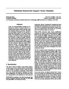
where x j and w j are components of the vectors x and w, respectively. Figure 1 shows a training sample that is linear separable, i.e. there exists a hyperplane that separates positive and negative objects. If the training set is linear separable, perceptron learning algorithm will find the vector w such that:
The authors would like to thank NSERC for their financial support.
0-7803-8376-1/04/$20.00 Copyright 2004 IEEE.
y × [ x, w + b ] ≥ 0 for all (x, y ) ∈ S .
(1)
Fig. 1. Linear Separable Sample (Source: Cristiani, 2003 [3])
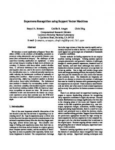
The dimensionality rises very quickly with the degree of polynomial. For example, Hoffmann (2002) report that for an original input space with 256 dimensions, the transformed space with second degree polynomials was approximately 33,000, and for the third degree polynomials the dimensionality was more than a million, and fourth degree led to a more than billion dimension space. This problem of high dimensionality will be discussed later in the paper. The original perceptron algorithm was used to find one of the possibly many hyperplanes separating two classes. The choice of the hyperplane was arbitrary. Support vector machines use the size of margin between two classes to search for the optimal hyperplane. Figure 3 shows the concept of margin between two classes.
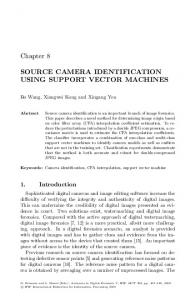
One of the major shortcomings [7] of the perceptron algorithm was that it was only applicable to training set that was linear separable. Neural network community tried to overcome this shortcoming by using one or more hidden layers and non-linear activation functions [6]. The support vector machines overcome the shortcomings of the linear separability in perceptron approach by using a mapping Φ of input space to another feature space with higher dimension as shown in figure 2. Equation (1) for perceptron is then changed to:
y × [ Φ (x), Φ (w ) + b ] ≥ 0 for all (x, y ) ∈ S .
(2) Fig. 3. Margin between two classes (Source: Cristianini, 2003 [3])
The problem of maximizing the margin can be reduced to an optimization problem [3,14]:
[
]
Minimize w, w such that y × x, w + b ≥ 0 for all (x, y ) ∈ S . Fig. 2. Non-linear separable feature space to linear separable feature space (Source: Cristiani, 2003 [3])
Usually, high dimensional transformation is needed in order to obtain reasonable classification [3]. Computational overhead can be reduced by not explicitly mapping the data to feature space, but just working out the inner product in that space. In fact, support vector machines use a kernel function K corresponding to the inner product in the transformed feature space as: K (x, w ) = Φ (x), Φ ( w ) . Polynomial kernel is one of the popular kernel functions. Let us derive the polynomial kernel function of degree 2 for two dimensional input space. Let x = ( x1 , x 2 ) and w = ( w1 , w2 ) .
K (x, w ) =
x, w 2
2
2
= ( x1 w1 + x2 w2 ) 2
2
2
= =
( x1 w1 + x2 w2 + 2 x1 w1 x2 w2 ) 2 2 2 2 x1 + x2 + 2 x1 x2 , w1 + w2 + 2 w1 w2
=
Φ(x), Φ(w )
(3)
Support vector machines attempt to find a solution to such an optimization problem. III. ROUGH SET THEORY The notion of rough set was proposed by Pawlak [9,10,11]. This section provides a brief summary of the concepts from rough set theory. Let U denote the universe (a finite ordinary set), and let
R ⊆ U × U be an equivalence (indiscernibility) relation on U. The pair A = (U, R) is called an approximation space.
The equivalence relation R partitions the set U into disjoint subsets. Such a partition of the universe is denoted by U/R = E1, E2... En, where Ei is an equivalence class of R. If two elements u, v ∈ U belong to the same equivalence class E ⊆ U/R, we say that u and v are indistinguishable. The equivalence classes of R are called the elementary or atomic sets in the approximation space A = (U, R). The union of one or more elementary sets is called a composed set in A. The empty set ∅ is also considered a special composed set. Com
Actual set
between the two classes. There are no training examples in the margin in Figure 3. The optimal hyperplane gives us the best possible dividing line. However, if one chooses to not make an assumption about the classification of objects in the margin, the margin can be designated as the boundary region. This will allow us to create rough sets as follows.
Upper approximation
Let us define b1 as follows: y × x, w + b1 ≥ 0 for all
An equivalence class Lower approximation
[
]
(x, y ) ∈ S , and there exists at least one training example (x, y ) ∈ S such that y = 1 and y × [ x, w + b1 ] = 0 . Fig. 4. Rough Set Approximation
(A) denotes the family of all composed sets. Since it is not possible to differentiate the elements within the same equivalence class, one may not be able to obtain a precise representation for an arbitrary set X ⊆ U in terms of elementary sets in A. Instead, its lower and upper bounds may represent the set X. The lower bound A (X) is the union of all the elementary sets, which are subsets of X. The upper bound
A (X) is the union of all the elementary sets that have a nonempty intersection with X. The pair ( A( X ), A( X )) is the representation of an ordinary set of X in the approximation space A = (U,R), or simply the rough set of X. The elements in the lower bound of X definitely belong to X, while elements in the upper bound of X may or may not belong to X. Figure 4 illustrates the lower and upper approximation. It can be verified, that for any subsets X, Y ⊆ U, the following lemmas hold [9].
A( X I Y ) = A( X ) I A(Y ), A( X U Y ) = A( X ) U A(Y ),
A( X I Y ) = A( X ) I A(Y ), A( X U Y ) = A( X ) U A(Y ), A(− X ) = − A( X ), A(− X ) = − A( X ), X ⊇ Y ⇒ ( A( X ) ⊇ A(Y ), A( X ) ⊇ A(Y )), A(U ) = A(U ) = U , A(0) = A(∅) = ∅, IV. ROUGH SETS BASED ON SUPPORT VECTOR MACHINE CLASSIFICATION We will first consider the ideal scenario, where the transformed feature space is linear separable and the SVM has found the optimal hyperplane by maximizing the margin
[
]
Similarly, b2 is defined as: y × x, w + b2 ≥ 0 for all
(x, y ) ∈ S , and there exists at least one training example (x, y ) ∈ S such that y = -1 and y × [ x, w + b2 ] = 0 . It can be easily seen that b1 and b2 correspond to the boundaries of the margin in Figure 3. The modified SVM classifier can then be defined as follows. If x, w + b1 ≥ 0 , classification of x is +1.
(R1)
If x, w + b2 ≤ 0 , classification of x is -1.
(R2)
Otherwise, classification of x is uncertain.
(R3)
The proposed classifier will allow us to create three equivalence classes, and define a rough set based approximation space. This simple extension of an SVM classifier provides a basis for a more practical application, when the SVM transformation does not lead to a linear separable case. Cristianini [3] list disadvantages of refining feature space to achieve linear separability. Often this will lead to high dimensions, which will increase the computational requirements significantly. Moreover, it is easy to overfit in high dimensional spaces, i.e. regularities could be found in the training set that are accidental, which would not be found again in a test set. The soft margin classifiers [3] modify the optimization problem to allow for an error rate. The rough set based rules given by (R1-R3) can still be used by empirically determining the values of b1 and b2 . For example, b1 can be chosen in such a way that for an
(x, y ) ∈ S if x, w + b1 ≥ 0 , then y must be +1, and b2 can be chosen in such a way that for an (x, y ) ∈ S if x, w + b2 ≤ 0 , then y must be -1. Assuming there are no outliers, such a choice of b1 and b2 would be reasonable. Otherwise, one can specify that the requirements hold for a significant percentage of training examples. For example, b1 can be chosen in such a way that for an
(x, y ) ∈ S if
x, w + b1 ≥ 0 , then in at least 95% of the cases y must be +1. Similarly, b2 can be chosen in such a way that for an
(x, y ) ∈ S if x, w + b2 ≤ 0 , then in at least 95% of the cases y must be -1. The proposed extension can be easily implemented after the soft margin classifier determines the value of w. All the objects in the training sample will be sorted based on the values of x, w . Value of b1 can be found by going down (or up if the positive examples are below the hyperplane) in the list until 95% of the positive examples are found. Value of b2 can be found by going up (or down if the positive examples are below the hyperplane) in the list until 95% of the negative examples are found.
REFERENCES [1] [2] [3] [4] [5] [6] [7] [8]
V. SUMMARY AND CONCLUSIONS This paper describes how a classification scheme obtained from a support vector machine (SVM) can be represented using rough or interval sets. The proposed extension is especially useful in practical situations when the feature space transformed by an SVM is not linear separable. If the dimensionality is increased, it may be possible to obtain a linear separable space. However, high dimensionality leads to higher computational requirements, and can also lead to overfitting of the classifier to training set. In such cases, soft margin classifiers are used by allowing a certain number of erroneous classifications. The paper describes how the hyperplane obtained by the soft margin classifier can be used to create a rough set based classification scheme.
[9] [10] [11] [12] [13] [14] [15] [16]
A. Hoffmann “VC Learning Theory and Support Vector Machines”, http://www.cse.unsw.edu.au/~cs9444/Notes02/Achim-Week11.pdf, 2003. N. Cristianini and J. Shawe-Taylor. An Introduction to Support Vector Machines (and other kernel-based learning methods), Cambridge University Press, 2000. N. Cristianini, “Support Vector and Kernel Methods for Pattern Recognition”, http://www.support-vector.net/tutorial.html, 2003. P-H. Chen, C-J. Lin, and B. Scholkopf, “A Tutorial on Support Vector Machines”, http://www.csie.ntu.edu.tw/~cjlin/papers/nusvmtutorial.pdf, 2002. A.F. 1. da Rocha, and R.R. Yager, “Neural Nets and Fuzzy Logic”, in Hybrid Architectures for Intelligent Systems, A. Kandel and G. Langholz, eds., CRC Press, Ann Arbor, 1992, pp. 3-28. R. Hecht-Nielsen, Neurocomputing, Addison-Wesley Publishing, Don Mills, Ontario, 1990. M. L. Minsky and S. A. Papert. Perceptrons. The MIT Press, Cambridge, MA, 1969. J. Platt, “Support Vector Machines”, http://research.microsoft.com/users/jplatt/svm.html, 2003. Z. Pawlak, “Rough sets”, International Journal of Information and Computer Sciences, vol. 11, 1982, pp. 145-172. Z. Pawlak, “Rough classification”, International Journal of ManMachine Studies, vol. 20, 1984, pp. 469-483. Z.Pawlak, Rough Sets: Theoretical Aspects of Reasoning about Data, Kluwer Academic Publishers, 1992. V. Vapnik, “Support-Vector Networks”, Machine Learning, vol. 20, issue 3, September 1995a, pp. 273-297. V. Vapnik. The Nature of Statistical Learning Theory. Springer Verlag, New York, 1995b. V. Vapnik. Statistical Learning Theory. Wiley, NY, 1998. V. Vapnik and O. Chapelle, “Bounds on error expectation for support vector machines”, NeuralComputation, vol. 12, issue 9, 2000, pp. 2013– 2036. F. Rosenblatt, “The perceptron: A perceiving and recognizing automaton”, Technical Report 85-460-1, Project PARA, Cornell Aeronautical Lab, 1957.