Intra-Option Learning about Temporally Abstract Actions
Richard S. Sutton Department of Computer Science University of Massachusetts Amherst, MA 01003-4610
[email protected]
Doina Precup Department of Computer Science University of Massachusetts Amherst, MA 01003-4610
[email protected]
Abstract Several researchers have proposed modeling temporally abstract actions in reinforcement learning by the combination of a policy and a termination condition, which we refer to as an option. Value functions over options and models of options can be learned using methods designed for semi-Markov decision processes (SMDPs). However, all these methods require an option to be executed to termination. In this paper we explore methods that learn about an option from small fragments of experience consistent with that option, even if the option itself is not executed. We call these methods intra-option learning methods because they learn from experience within an option. Intra-option methods are sometimes much more efficient than SMDP methods because they can use off-policy temporaldifference mechanisms to learn simultaneously about all the options consistent with an experience, not just the few that were actually executed. In this paper we present intra-option learning methods for learning value functions over options and for learning multi-time models of the consequences of options. We present computational examples in which these new methods learn much faster than SMDP methods and learn effectively when SMDP methods cannot learn at all. We also sketch a convergence proof for intraoption value learning.
1 Introduction Learning, planning, and representing knowledge at multiple levels of temporal abstraction remain key challenges for AI. Recently, several researchers have begun to address
Satinder Singh Department of Computer Science University of Colorado Boulder, CO 80309-0430
[email protected]
these challenges within the framework of reinforcement learning and Markov decision processes (MDPs) (e.g., Singh, 1992a,b; Kaelbling, 1993; Lin, 1993; Dayan & Hinton, 1993; Thrun and Schwartz, 1995; Sutton, 1995; Huber and Grupen, 1997; Kalm´ar, Szepesv´ari, and L¨orincz, 1997; Dietterich, 1998; Parr and Russell, 1998; Precup, Sutton, and Singh 1997, 1998a,b). This framework is appealing because of its general goal formulation, applicability to stochastic environments, and ability to use sample or simulation models (e.g., see Sutton and Barto, 1998). Extensions of MDPs to semi-Markov decision processes (SMDPs) provide a way to model temporally abstract actions, as we summarize in Sections 3 and 4 below. Common to much of this recent work is the modeling of a temporally extended action as a policy (controller) and a condition for terminating, which we together refer to as an option. Options are a flexible way of representing temporally extended courses of action such that they can be used interachangeably with primitive actions in existing learning and planning methods (Sutton, Precup, and Singh, in preparation). In this paper we explore ways for learning about options using a class of off-policy, temporal-difference methods that we call intra-option learning methods. Intra-option methods look inside options to learn about them even when only a single action is taken that is consistent with them. Whereas SMDP methods treat options as indivisible black boxes, intra-option methods attempt to take advantage of their internal structure to speed learning. Intraoption methods were introduced by Sutton (1995), but only for a pure prediction case, with a single policy. The structure of this paper is as follows. First we introduce the basic notation of reinforcement learning, options and models of options. In Section 4 we briefly review SMDP methods for learning value functions over options and thus how to select among options. Our new results are in Sections 5–7. Section 5 introduces an intra-option method for
learning value functions and sketches a proof of its convergence. Computational experiments comparing it with SMDP methods are presented in Section 6. Section 7 concerns methods for learning models of options, as are used in planning: we introduce an intra-option method and illustrate its advantages in computational experiments.
The action value functions satisfy the Bellman equations:
2 Reinforcement Learning (MDP) Framework
3 Options
In the reinforcement learning framework, a learning agent interacts with an environment at some discrete, lowest-level time scale . At each time step, the agent , and on that perceives the state of the environment, basis chooses a primitive action, . In response to , the environment produces one step later a numerical reward, , and a next state, . We denote the union of the action sets by . If and , are finite, then the environment’s transition dynamics are modeled by one-step state-transition probabilities, and onestep expected rewards, Pr
and
for all
and (it is understood here that for ). These two sets of quantities together constitute the one-step model of the environment. The agent’s objective is to learn a policy , which is a mapping from states to probabilities of taking each action, that maximizes the expected discounted future reward from each state :
where
is a discount-rate parameter. The quantity is called the value of state under policy , and is called the value function for policy . The optimal value of a state is denoted
Particularly important for learning methods is a parallel set of value functions for state–action pairs rather than for states. The value of taking action in state under policy , denoted , is the expected discounted future reward starting in , taking , and henceforth following :
This is known as the action-value function for policy . The optimal action-value function is
(1) (2)
We use the term options for our generalization of primitive actions to include temporally extended courses of action. In this paper, we focus on Markov options, which consist of three components: a policy , a termination condition , and an input set . An option is available in state if and only if . If the option is taken, then actions are selected according to until the option terminates stochastically according to . In particular, if the option taken in state is Markov, then the next action is selected according to the probability distribution . The environment then makes a transition to , where the option either terminates, with probastate bility , or else continues, determining according to , possibly terminating in according to , and so on. When the option terminates, then the agent has the opportunity to select another option. The input set and termination condition of an option together restrict its range of application in a potentially useful way. In particular, they limit the range over which the option’s policy needs to be defined. For example, a handcrafted policy for a mobile robot to dock with its battery charger might be defined only for states in which the battery charger is within sight. The termination condition would be defined to be outside of and when the robot is successfully docked. For Markov options it is natural to assume that all states where an option might continue are also states where the option might be taken (i.e., that ). In this case, needs to be defined only over rather than over all of . Given a set of options, their input sets implicitly define a for each state . The sets set of available options are much like the sets of available actions, . We can unify these two kinds of sets by noting that actions can be considered a special case of options. Each action corresponds to an option that is available whenever is available ( ), that always lasts exactly one step ( ), and that selects everywhere ). Thus, we can consider the agent’s ( choice at each time to be entirely among options, some of which persist for a single time step, others which are more temporally extended. We refer to the former as one-step or primitive options and the latter as multi-step options.
We now consider Markov policies over options, , and their value functions. When initiated in a state , such a policy selects an option according to probability distribution . The option is taken in , determining actions until it terminates in , at which point a new option is selected, according to , and so on. In this way a policy over options, , determines a policy over actions, or flat policy, . Henceforth we use the unqualified term policy for Markov policies over options, which include Markov flat policies as a special case. Note, however, that is typically not Markov because the action taken in a state depends on which option is being taken at the time, not just on the state. We define the value of a state under a general flat policy as the expected return if the policy is started in :
where denotes the event of being initiated in at time . The value of a state under a general policy (i.e., a policy over options) can then be defined as the value of the state under the corresponding flat policy: . It is natural to also generalize the action-value function to an option-value function. We define , the value of under policy , as taking option in state
where , the composition of and , denotes the policy that first follows until it terminates and then initiates in the resultant state.
state-prediction part of the model of for state is Pr (4) for all , under the same conditions, where is an identity indicator, equal to 1 if , and equal to 0 else. Thus, is a combination of the likelhood that is the state in which terminates together with a measure of how delayed that outcome is relative to . We call this kind of model a multi-time model because it describes the outcome of an option not at a single time but at potentially many different times, appropriately combined.
4 SMDP Learning Methods Using multi-time models of options we can write Bellman equations for general policies and options. For example, the Bellman equation for the value of option in state under a Markov policy is (5) The optimal value functions and optimal Bellman equations can also be generalized to options and to policies over options. Of course, the conventional optimal value funcand are not affected by the introduction of tions options; one can ultimately do just as well with primitive actions as one can with options. Nevertheless, it is interesting to know how well one can do with a restricted set of options that does not include all the actions. For example, one might first consider only high-level options in order to find an approximate solution quickly. Let us denote the restricted set of options by and the set of all policies that select only from by . Then the optimal value function given that we can select only from is
Options are closely related to the actions in a special kind of decision problem known as a semi-Markov decision process, or SMDP (e.g., see Puterman, 1994). Any fixed set of options for a given MDP defines a new SMDP overlaid on the MDP. The appropriate form of model for options, and defined earlier for actions, is analogous to the known from existing SMDP theory. For each state in which an option may be started, this kind of model predicts the state in which the option will terminate and the total reward received along the way. These quantities are discounted in a particular way. For any option , let denote the event of being taken in state at time . Then the reward part of the model of for state is
denotes the event of starting the execution where of option in state , is the random numbner opf steps elapsing during , is the resulting next state, and is the cumulative discounted reward received along the way. The optimal option values are defined as:
(3)
(8)
is the random time at which terminates. The
(9)
where
(6) (7)
Given a set of options, , a corresponding optimal pol, is any policy that achieves , i.e., for icy, denoted which for all states . If and models of the options are known, then optimal policies can be formed by choosing in any proportion among the maximizing options in (7). Or, if is known, then optimal policies can be formed by choosing in each state in any proportion among the options for which . Thus, computing approximations to or become the primary goals of planning and learning methods with options. The problem of finding the optimal value functions for a set of options can be addressed by learning methods. Because an MDP augmented by options forms an SMDP, we can apply SMDP learning methods as developed by Bradtke and Duff (1995), Parr and Russell (1998), Parr (in preparation), Mahadevan et al. (1997), and McGovern, Sutton and Fagg (1997). In these methods, each option is viewed as an indivisible, opaque unit. After the execution of option is started in state , we next jump to the state in which it terminates. Based on this experience, an estimate of the optimal option-value function is updated. For example, the SMDP version of one-step Q-learning (Bradtke and Duff, 1995), which we call one-step SMDP Q-learning, updates after each option termination by
where is the number of time steps elapsing between and , is the cumulative discounted reward over this time, and it is implicit that the step-size parameter may depend arbitrarily on the states, option, and time steps. The estimate converges to for all and under conditions similar to those for conventional Q-learning (Parr, in preparation).
5 Intra-Option Value Learning One drawback to SMDP learning methods is that they need to execute an option to termination before they can learn about it. Because of this, they can only be applied to one option at a time—the option that is executing at that time. More interesting and potentially more powerful methods are possible by taking advantage of the structure inside each option. In particular, if the options are Markov and we are willing to look inside them, then we can use special temporal-difference methods to learn usefully about an option before the option terminates. This is the main idea behind intra-option methods. Intra-option methods are examples of off-policy learning methods (Sutton and Barto, 1998) in that they learn about
the consequences of one policy while actually behaving according to another, potentially different policy. Intra-option methods can be used to learn simultaneously about many different options from the same experience. Moreover, they can learn about the values of executing options without ever executing those options. Intra-option methods for value learning are potentially more efficient than SMDP methods because they extract more training examples from the same experience. For example, suppose we are learning to approximate and that is Markov. Based on an execution of from to , SMDP methods extract a single training example for . But because is Markov, it is, in a sense, also initiated at each of the steps between and . The jumps to are also valid experifrom each intermediate ences with , experiences that can be used to improve estimates of . Or consider an option that is very similar to and which would have selected the same actions, but which would have terminated one step later, at rather than at . Formally this is a different option, and formally it was not executed, yet all this experience could be used for learning relevant to it. In fact, an option can often learn something from experience that is only slightly related (occasionally selecting the same actions) to what would be generated by executing the option. This is the idea of off-policy training—to make full use of whatever experience occurs in order to learn as much possible about all options, irrespective of their role in generating the experience. To make the best use of experience we would like an off-policy and intra-option version of Q-learning. It is convenient to introduce new notation for the value of a state–option pair given that the option is Markov and executing upon arrival in the state:
Then we can write Bellman-like equations that relate to expected values of , where is the immediate successor to after initiating Markov option in :
where is the immediate reward upon arrival in . Now consider learning methods based on this Bellman equation. Suppose action is taken in state to produce next state and reward , and that was selected in a way consistent with the Markov policy of an option
. That is, suppose that was selected accord. Then the Bellman equation ing to the distribution above suggests applying the off-policy one-step temporaldifference update:
4 stochastic primitive actions
HALLWAYS
up left
o1
G
where o2
The method we call one-step intra-option Q-learning applies this update rule to every option consistent with every action taken . Theorem 1 (Convergence of intra-option Q-learning) For any set of deterministic Markov options , one-step intra-option Q-learning converges w.p.1 to the optimal Q-values, , for every option, regardless of what options are executed during learning, provided every primitive action gets executed in every state infinitely often. , for every opProof: (Sketch) On experiencing tion that picks action in state , intra-option Q-learning performs the following update:
Let be the action selection by deterministic Markov option . Our result follows directly from Theorem of Jaakkola et al. (1994) and the observation that the expected value of the update operator yields a contraction, as shown below:
*
right
Fail 33% of the time
down
8 multi-step options (to each room's 2 hallways)
Figure 1: The rooms example is a gridworld environment with stochastic cell-to-cell actions and room-to-room hallway options. Two of the hallway options are suggested by the arrows labeled and . The label indicates the location used as a goal.
the grid correspond to the states of the environment. From any state the agent can perform one of four actions, up, down, left or right, which have a stochastic effect. With probability 2/3, the actions cause the agent to move one cell in the corresponding direction, and with probability 1/3, the agent moves instead in one of the other three directions, each with 1/9 probability. If the movement would take the agent into a wall, then the agent remains in the same cell. There are small negative rewards for each action, with means uniformly distributed between 0 and -1. The rewards are also perturbed by gaussian noise with standard deviation 0.1. The environment also has a goal state, labeled “G”. A complete trip from a random start state to the goal state is called an episode. When the agent enters “G”, it gets a reward of and the episode ends. In all the experiments the discount parameter was and all the initial value estimates were . In each of the four rooms we provide two built-in hallway options designed to take the agent from anywhere within the room to one of the two hallway cells leading out of the room. The policies underlying the options follow the shortest expected path to the hallway.
6 Illustrations of Intra-Option Value Learning As an illustration of intra-option value-learning, we used the gridworld environment shown in Figure 1. The cells of
For the first experiment, we applied the intra-option method in this environment without selecting the hallway options. In each episode, the agent started at a random state in the environment and thereafter selected primitive actions randomly, with equal probability. On every transition, the update (5) was applied first to the primitive action taken, then to any of the hallway options that were consistent with it. The hallway options were updated in clockwise order, starting from any hallways that faced up from the current state. . The value of the step-size parameter was This is a case in which SMDP methods would not be able to
3.5
Value of optimal policy 3
-2
Absolute error in option values averaged over the options
2.5
Average value of greedy policy
-3
2 1.5
SMDP Q-learning
1
Macro Q-learning -4
0.5
1
10
100
1000
0
6000
Intra 0
2000
4000
6000
8000
10000
8000
10000
Episodes
Episodes -2
0
-2.2
Learned value
-1
Upper hallway option
True value
-2 Learned value
Option values for *
1000
Left hallway option 2000
3000
-2.6
Macro Q-learning
-2.8
Intra-option value learning
-3
-3.4
True value
0
Average on-line reward
-3.2
-3
-4
SMDP Q-learning
-2.4
4000
5000
6000
-3.6 -3.8 -4
0
2000
Figure 2: The learning of option values by intra-option methods without ever selecting the options. The value of the greedy policy goes to the optimal value (upper panel) as the learned values approach the correct values (as shown for one state, in the lower panel). learn anything about the hallway options, because these options are never executed. However, the intra-option method learned the values of these actions effectively, as shown in Figure 2. The upper panel shows the value of the greedy policy learned by the intra-option method, averaged over and over 30 repetitions of the whole experiment. The lower panel shows the correct and learned values for the two hallway options that apply in the state marked in Figure 1. Similar convergence to the true values was observed for all the other states and options. So far we have illustrated the effectiveness of intra-option learning in a context in which SMDP methods do not apply. How do intra-option methods compare to SMDP methods when both are applicable? In order to investigate this question, we used the same environment, but now we allowed the agent to choose among the hallway options as well as the primitive actions, which were treated as onestep options. In this case, SMDP methods can be ap-
4000
6000
Episodes
Episodes
Figure 3: Comparison of SMDP, intra-option and macro Qlearning. Intra-option methods converge faster to the correct values. plied, since all the options are actually executed. We experimented with two SMDP methods: one-step SMDP Qlearning (Bradtke and Duff, 1995) and a hierarchical form of Q-learning called macro Q-learning (McGovern, Sutton and Fagg, 1997). The difference between the two methods is that, when taking a multi-step option, SMDP Q-learning only updates the value of that option, whereas macro Qlearning also updates the values of the one-step options (actions) that were taken along the way. In this experiment, options were selected not at random, but in an -greedy way dependent on the current option-value estimates. That is, given the current estimates , let denote the best valued action (with ties broken randomly). Then the policy used to select options was if otherwise, for all and action, , was set at
. The probability of a random in all cases. For each algorithm,
we tried step-size values of picked the best one.
, and
and then
Figure 3 shows two measures of the performance of the learning algorithms. The upper panel shows the average for the hallway opabsolute error in the estimates of tions, averaged over the input sets , the eight hallway options, and 30 repetitions of the whole experiment. The intra-option method showed significantly faster learning than any of the SMDP methods. The lower panel shows the quality of the policy executed by each method, measured as the average reward over the state space. The intra-option method was also the fastest to learn by this measure.
is related to itself by (12)
(13) where and are the reward and next state given that action is taken in state , and
7 Intra-Option Model Learning In this section, we consider intra-option methods for learn, given knowling multi-time models of options, and edge of the option (i.e., of its , , and ). Such models are used in planning methods (e.g., Precup, Sutton, and Singh, 1997, 1998a,b). The most straightforward approach to learning the model of an option is to execute the option to termination many times in each state , recording the resultant next states , cumulative discounted rewards , and elapsed times . These outcomes can then be averaged to approximate the expected values for and given by (3) and (4). For example, an incremental learning rule for this could update its estimates and , for all , after each execution of in state , by and
(10) (11)
where the step-size parameter, , may be constant or may depend on the state, option, and time. For example, if is 1 divided by the number of times that has been experienced in , then these updates maintain the estimates as sample averages of the experienced outcomes. However the averaging is done, we call these SMDP model-learning methods because, like SMDP value-learning methods, they are based on jumping from initiation to termination of each option, ignoring what might happen along the way. In the special case in which is a primitive action, note that SMDP model-learning methods reduce exactly to those used to learn conventional one-step models of actions. Now let us consider intra-option methods for model learning. The idea is to use Bellman equations for the model, just as we used the Bellman equations in the case of learning value functions. The correct model of a Markov option
for all . How can we turn these Bellman equations into update rules for learning the model? First consider that action is taken in and that the way it was selected is consistent with , that is, that was selected with the distribution . Then the Bellman equations above suggest the temporal-difference update rules (14) and
(15) where and are the estimates of and , respectively, and is a positive step-size parameter. The method we call one-step intra-option model learning applies these updates to every option consistent with every action taken. Of course, this is just the simplest intra-option model-learning method. Others may be possible using eligibility traces and standard tricks for off-policy learning (see Sutton, 1995; Sutton and Barto, 1998). Intra-option methods for model learning have advantages over SMDP methods similar to those we saw earlier for value-learning methods. As an illustration, consider the application of SMDP and intra-option model-learning methods to the rooms example. We assume that the eight hallway options are given as before, but now we assume that their models are not given and must be learned. Experience is generated by selecting randomly in each state among the two possible options and four possible actions, with no goal state. In the SMDP model-learning method, equations (10) and (11) were applied whenever an option was selected, whereas, in the intra-option model-learning method, equations (14) and (15) were applied on every step to all options that were consistent with the action taken on that step. In this example, all options are deterministic, so consistency
8 Closing
Reward prediction error
4
Max error 3
SMDP Intra
SMDP 1/t
2
Avg. error 1
SMDP Intra
0
0
20,000
SMDP 1/t 40,000
60,000
80,000
100,000
The theoretical and empirical results presented in this paper suggest that intra-option methods provide an efficient way for taking advantage of the structure inside an option. Intra-option methods use experience with a single action to update the value or model for all the options that are consistent with that action. In this way they make much more efficient use of the experience than SMDP methods, which treat options as indivisible units. In the future, we plan to extend these algorithms for the case of non-Markov options, and to combine them with eligibility traces.
Options executed
Acknowledgements 0.7
State prediction error
0.6 0.5 0.4
SMDP
0.3
SMDP 1/t
0.2
0
Intra
SMDP 1/t
0.1
SMDP
Intra 0
20,000
40,000
60,000
80,000
Max error Avg. error 100,000
Options executed
Figure 4: Learning curves for model learning by SMDP and intra-option methods.
The authors acknowledge the help of their the colleagues Amy McGovern, Andy Barto, Csaba Szepesv´ari, Andr´as L¨orincz, Ron Parr, Tom Dietterich, Andrew Fagg, Leo Zelevinsky and Manfred Huber. We also thank Andy Barto, Paul Cohen, Robbie Moll, Mance Harmon, Sascha Engelbrecht, and Ted Perkins for helpful reactions and constructive criticism. This work was supported by NSF grant ECS9511805 and grant AFOSR-F49620-96-1-0254, both to Andrew Barto and Richard Sutton. Doina Precup also acknowledges the support of the Fulbright foundation. Satinder Singh was supported by NSF grant IIS-9711753.
References Bradtke, S. J. & Duff, M. O. (1995). Reinforcement learning methods for continuous-time Markov decision problems. In Advances in Neural Information Processing Systems 7 (pp. 393–400). MIT Press.
with the action selected means simply that the option would have selected that action. For the SMDP method, the step-size parameter was varied so that the model estimates were sample averages, which should give fastest learning. The results of this method are labeled “SMDP 1/t” on the graphs. We also looked at results using a fixed learning rate. In this case and for the intra-option method we tried step-size values of , and , and picked the best value for each method. Figure 4 shows the learning curves for all three methods, using the best values, when a fixed alpha was used. The upper panel shows the average and maximum absolute error in the reward predictions, and the lower panel shows the average absolute error and the maximum absolute error in the transition predictions, averaged over the eight options and over 30 independent runs. The intraoption method approached the correct values more rapidly than the SMDP methods.
Dayan, P. & Hinton, G. E. (1993). Feudal reinforcement learning. In Advances in Neural Information Processing Systems 5 (pp. 271–278). Morgan Kaufmann. Dietterich, T. G. (1998). The MAXQ method for hierarchical reinforcement learning. In Proceedings of the Fifteenth International Conference on Machine Learning. Morgan Kaufmann. Huber, M. & Grupen, R. A. (1997). A feedback control structure for on-line learning tasks. Robotics and Autonomous Systems, 22(3-4), 303–315. Jaakkola, T., Jordan, M. & Singh, S. (1994). On the convergence of stochastic iterative dynamic programming algorithms. Neural Computation, 6(6), 1185–1201. Kaelbling, L. P. (1993). Hierarchical learning in stochastic domains: Preliminary results. In Proceedings of the
Tenth International Conference on Machine Learning (pp. 167–173). Morgan Kaufmann. Kalm´ar, Z., Szepesv´ari, C. & L¨orincz, A. (1997). Module based reinforcement learning for a real robot. In Proceedings of the Sixth European Workshop on Learning Robots (pp. 22–32). Lin, L.-J. (1993). Reinforcement Learning for Robots Using Neural Networks. PhD thesis, Carnegie Mellon University. Mahadevan, S., Marchallek, N., Das, T. K. & Gosavi, A. (1997). Self-improving factory simulation using continuous-time average-reward reinforcement learning. In Proceedings of the Fourteenth International Conference on Machine Learning (pp. 202– 210). Morgan Kaufmann. McGovern, A., Sutton, R. S. & Fagg, A. H. (1997). Roles of macro-actions in accelerating reinforcement learning. In Grace Hopper Celebration of Women in Computing (pp. 13–17). Parr, R. (in preparation). Hierarchical Control and learning for Markov decision processes. PhD thesis, Berkeley University. Chapter 3. Parr, R. & Russel, S. (1998). Reinforcement learning with hierarchies of machines. In Advances in Neural Information Processing Systems 10. MIT Press. Precup, D., Sutton, R. S. & Singh, S. (1997). Planning with closed-loop macro actions. In Working Notes of the AAAI Fall Symposium ’97 on Model-directed Autonomous Systems (pp. 70–76). Precup, D., Sutton, R. S. & Singh, S. (1998a). Multi-time models for temporally abstract planning. In Advances in Neural Information Processing Systems 10. MIT Press. Precup, D., Sutton, R. S. & Singh, S. (1998b). Theoretical results on reinforcement learning with temporally abstract options. In Machine Learning: ECML98. 10th European Conference on Machine Learning, Chemnitz, Germany, April 1998. Proceedings (pp. 382– 393). Springer Verlag. Puterman, M. L. (1994). Markov Decision Processes: Discrete Stochastic Dynamic Programming. Wiley. Singh, S. P. (1992a). Reinforcement learning with a hierarchy of abstract models. In Proceedings of the Tenth National Conference on Artificial Intelligence (pp. 202–207). MIT/AAAI Press.
Singh, S. P. (1992b). Scaling reinforcement learning by learning variable temporal resolution models. In Proceedings of the Ninth International Conference on Machine Learning (pp. 406–415). Morgan Kaufmann. Sutton, R. S. (1995). TD models: Modeling the world as a mixture of time scales. In Proceedings of the Twelfth International Conference on Machine Learning (pp. 531–539). Morgan Kaufmann. Sutton, R. S. & Barto, A. G. (1998). Reinforcement Learning: An Introduction. MIT Press. Sutton, R. S., Precup, D. & Singh, S. (in preparation). Between MDPs and Semi-MDPs: learning, planning, and representing knowledge at multiple temporal scales. Journal of AI Research. Thrun, S. & Schwartz, A. (1995). Finding structure in reinforcement learning. In Advances in Neural Information Processing Systems 7 (pp. 385–392). MIT Press.