stable learning algorithm for blind separation of temporally ... - CiteSeerX

4th International Symposium on Independent Component Analysis and Blind Signal Separation (ICA2003), April 2003, Nara, Japan

STABLE LEARNING ALGORITHM FOR BLIND SEPARATION OF TEMPORALLY CORRELATED SIGNALS COMBINING MULTISTAGE ICA AND LINEAR PREDICTION Tsuyoki NISHIKAWA Hiroshi SARUWATARI Kiyohiro SHIKANO Graduate School of Information Science, Nara Institute of Science and Technology 8916-5 Takayama-cho, Ikoma-shi, Nara, 630-0192, JAPAN E-mail: {tsuyo-ni, sawatari, shikano}@is.aist-nara.ac.jp the stability of learning cannot be guaranteed. In order to solve both problems simultaneously, we propose the novel approach in which the linear predictors estimated from the roughly separated source signals by FDICA are inserted before TDICA with a holonomic constraint as a prewhitening processing (after TDICA, the dewhitening is also performed). The stability of the learning in TDICA can be guaranteed by the holonomic constraint, and it is still possible to separate the temporally correlated signals because the pre/dewhitening processing prevents the ICA from performing the decorrelation. The experimental results under a reverberant condition reveal that the proposed algorithm results in the higher stability and higher separation performance than the conventional MSICA.

ABSTRACT We newly propose a stable algorithm for blind source separation (BSS) combining multistage ICA (MSICA) and linear prediction. The MSICA is the method previously proposed by the authors, in which frequency-domain ICA (FDICA) for a rough separation is followed by time-domain ICA (TDICA) to remove residual crosstalk. For temporally correlated signals, we must use TDICA with a nonholonomic constraint to avoid the decorrelation effect from the holonomic constraint. However, the stability cannot be guaranteed in the nonholonomic case. To solve the problem, the linear predictors estimated from the roughly separated signals by FDICA are inserted before the holonomic TDICA as a prewhitening processing, and the dewhitening is performed after TDICA. The stability of the proposed algorithm can be guaranteed by the holonomic constraint, and the pre/dewhitening processing prevents the decorrelation. The experiments in a reverberant room reveal that the algorithm results in higher stability and separation performance.

2. SOUND MIXING MODEL OF MICROPHONE ARRAY In general, the observed signals in which multiple source signals are convoluted with room impulse responses are obtained by the following equation: P −1 X x(t) = a(τ )s(t − τ ), (1)

1. INTRODUCTION

τ =0

where x(t) = [x1 (t), · · · , xK (t)]T is the observed signal vector and s(t) = [s1 (t), · · · , sL (t)]T is the source signal vector (see Fig. 1) . K is the number of array elements (microphones) and L is the number of multiple sound sources. In this study, we deal with the case of K = L = 2. Also, a(τ ) = [aij (τ )]ij ([·]ij denotes the matrix in which ij-th element is [·]) is the mixing filter matrix. P is the length of the impulse response which is assumed to be an FIR-filter of thousands of taps because we introduce a model to deal with the arrival lags among the elements of the microphone array and the room reverberations.

Blind source separation (BSS) is an approach for estimating original source signals only from the information of the mixed signals observed in each input channel. This technique is applicable to high-quality hand-free speech recognition systems. Many BSS methods based on independent component analysis (ICA) [1] have been proposed [2, 3, 4] for the acoustic signal separation. However, the performances of these methods degrade seriously, especially under heavily reverberant conditions. In order to improve the separation performance, we have proposed an efficient BSS algorithm called multistage ICA (MSICA), in which frequency-domain ICA (FDICA) [3, 5] and time-domain ICA (TDICA) [2, 6] are combined [7]. In this method, first, FDICA can find an approximate solution to separate the sources to a certain extent, and finally TDICA can remove the residual crosstalk components from FDICA. Therefore, the improvement of TDICA is a primary issue because the quality of resultant separated signals is determined by TDICA. In this paper, we discuss the stability of the TDICA algorithm, and newly propose a stable algorithm combining MSICA and linear prediction for temporally correlated signals, e.g., speech signals. First, the following points are explicitly noted: (1) The stability of learning in conventional TDICA with a holonomic constraint [6] is highly acceptable. However, the method cannot work well for speech signals due to the deconvolution property; i.e., the separated speech is harmfully distorted by the whitening process. (2) To decrease the whitening effect, TDICA with a nonholonomic constraint has been proposed [8]. This method, however, includes the inherent drawback that

3. CONVENTIONAL ICA AND PROBLEMS 3.1. Conventional FDICA and TDICA FDICA has the following advantages and disadvantages. Advantages: (F1) It is easy to converge the separation filter in iterative ICA learning because we can simplify the convolutive mixture down to simultaneous mixtures by the frequency transform. Disadvantages: (F2) The separation performance is saturated before reaching a sufficient performance level because the independence assumption collapses in each narrow-band [9]. (F3) Permutation among source signals and indeterminacy of each source gain in each subband.

337

Source signals

Mixing system

s 1 (t)

x1 (t)

a(τ) s 2 (t)

Observed signals

x2 (t)

Separated signals from FDICA

FDICA

z 1 (t)

Nonholonomic

The selection of TDICA is an important issue because the quality of resultant separated signals is determined by TDICA. We have two choices for TDICA algorithms; TDICA with a holonomic constraint [6] and TDICA with a nonholonomic constraint [8]. In the next section, detailed explanations for each algorithm and their problems are described.

Separated signals

y1 (t)

z 2 (t) TDICA y2 (t)

x(t) = Σ a(τ)s(t-τ) z(t)=IDFT[W(f)X(f,t)] τ

y(t) = Σ w (τ)z(t-τ) τ (NH)

3.3. Conventional TDICA with Holonomic Constraint

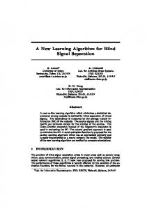
Fig. 1. Blind source separation procedure performed in the original MSICA [7]. In this system, the NH-TDICA is introduced to separate the temporally correlated signals by utilizing the flexibility of the nonholonomic constraint.

Amari proposed the TDICA algorithm which optimizes the separation filter by minimizing the Kullback-Leibler divergence (KLD) between the joint probability density function and the marginal probability density function of the separated signals [6]. The iterative equation of the separation filter w(H) (τ ) to minimize the KLD is given as (hereafter we designate the iterative equation as “H-TDICA”): [H-TDICA] Q−1n X (H) w(H) (τ ) = w (τ ) + α I δ(τ − d) i+1 i d=0 o (H) − h(y (t))y (t − τ + d)T it wi (d), (3)

Regarding the disadvantage (F3), various solutions have already been proposed [3, 10, 4, 11]. However, the collapse of the independence assumption, (F2), is a serious and inherent problem, and this prevents us from applying FDICA in a real acoustic environment with a long reverberation. TDICA has the following advantages and disadvantages. Advantages: (T1) We can treat the fullband speech signals where the independence assumption of sources usually holds.

where h·it denotes the time-averaging operator, i is used to express the value of the i-th step in the iterations, α is the step-size parameter and I is the identity matrix. δ(τ ) is Dirac delta function, where δ(0) = 1 and δ(n) = 0 (n 6= 0). Also, we define the nonlinear vector function (y (t)) ≡ tanh(y1 (t)), · · · , tanh(yL (t))]T .

Disadvantages: (T2) The convergence degrades under reverberant conditions because the iterative rule for FIR-filter learning is complicated.

3.4. Conventional TDICA with Nonholonomic Constraint

It is known that TDICA works only in the case of mixtures with a short-tap FIR filter, i.e., less than 100 taps. Also, TDICA fails to separate source signals under real acoustic environments because of the disadvantages (T2).

The H-TDICA forces the separated signals to have the characteristic that their higher-order autocorrelation is δ(τ ), i.e., the signals are temporally decorrelated. This performance might have a negative influence on the source separation. In order to solve the problem, Choi proposed a modified TDICA algorithm with a nonholonomic constraint [8]. In this algorithm, the constraint for the diagonal component of {·} part in Eq. (3), i.e., the higher-order autocorrelation of separated signals, is set to be arbitrary. The iterative equation of the separation filter w(NH) (τ ) is given as (hereafter we designate the iterative equation as “NH-TDICA”): [NH-TDICA]

3.2. BSS Algorithm Based on MSICA [7] As described above, the conventional ICA methods have some disadvantages. However, the advantages and disadvantages of FDICA and TDICA are mutually complementary, i.e., (F2) can be resolved by (T1), and (T2) can be resolved by (F1). Hence, in order to resolve the disadvantages, we have proposed a new algorithm, MSICA, in which FDICA and TDICA are cascaded (see Fig. 1). MSICA is conducted in the following steps. In the first stage, we perform FDICA to separate the source signals to some extent with the advantage of high stability. In the second stage, we regard the separated signals z (t) from FDICA as the input signals for TDICA, and we can remove the residual crosstalk components of FDICA by using TDICA. Finally, we regard the output signals from TDICA as the resultant separated signals. The separated signals of MSICA can be given as

y(t) =

Q−1

X

w(τ )z(t − τ ),

w(NH) i+1 (τ )

=

w(NH) (τ ) i

diag h(y (t))y (t − τ + d)T it d=0 o (NH) −h(y (t))y (t − τ + d)T it wi (d). (4)

+α

Q−1n

X

We have also introduced Eq. (4) in the original MSICA [7] to separate the mixed speech which corresponds to the temporally correlated signal by utilizing the flexibility of the nonholonomic constraint.

(2)

τ =0

3.5. Problems in Conventional TDICAs

where y (t) = [y1 (t), · · · , yL (t)] is the resultant separated signal vector of MSICA and z (t) = [z1 (t), · · · , zL (t)]T is the input signal vector for the TDICA part in MSICA (i.e., the output signals from FDICA). Also, w(τ ) = [wij (τ )]ij is the separation filter matrix, and Q is the length of the separation filter. In this procedure, we optimize w(τ ) so that the separated signals are mutually independent. T

The advantage and disadvantage of conventional TDICAs can be summarized as follows. (1) The stability of learning in H-TDICA is satisfactory. However, the method cannot work well for speech signals due to the deconvolution property; i.e., the separated speech is harmfully distorted by the whitening process. (2) On the other hand, NH-TDICA possibly performs no deconvolution, i.e., NHTDICA is applicable to speech signals. This method, however,

338

Source signals

Mixing system

s 1 (t) a(τ) s 2 (t)

Observed signals

x1 (t) x2 (t)

LP Coefficients p1(n)

Separated signals from FDICA

FDICA

LP

z 1 (t) z 2 (t)

LP

e1 (t) e2 (t)

v1 (t)

Holonomic

TDICA v (t) 2

Separated signals

DW DW

y1 (t) y2 (t)

v(t) = Σ w (τ)e(t-τ) τ (H)

LP: Linear predictor DW: Dewhitening processor

LP Coefficients p2(n)

Fig. 2. Blind source separation procedure performed in the proposed algorithm combining MSICA and linear prediction. In this system, the stability of the learning in TDICA can be guaranteed by the holonomic constraint, and it is still possible to separate the temporally correlated signals because the pre/dewhitening processing prevents the ICA from performing the decorrelation. where rl (τ ) = hzl (t)zl (t − τ )it is the autocorrelation of zl (t). Solving Eq. (6) basically involves the inversion of the matrix on the left-hand side. However, this can be simplified because the matrix is Toeplitz, i.e., all elements on each superdiagonal are equal and all elements on each subdiagonal are equal. Based on this property, we can easily and efficiently determine pl (n) by using LevinsonDurbun’s recursive algorithm [12]. The whitened signal el (t) is obtained by convolving the linear prediction coefficient pl (n) with zl (t) as

includes the inherent drawback that the stability of learning cannot be guaranteed as described in Sect. 5.4. Thus, the separation of temporally correlated signals such as speech cannot be achieved only using the conventional TDICAs. 4. PROPOSED ALGORITHM COMBINING MSICA AND LINEAR PREDICTION This section describes a new stable algorithm combining the linear prediction technique with an original MSICA (see Fig. 1). In the proposed algorithm, the linear predictors estimated from the roughly separated source signals by FDICA are inserted before TDICA with a holonomic constraint as a prewhitening processing (see Fig. 2). After TDICA, the dewhitening is also performed. The stability of the learning in TDICA can be guaranteed by the holonomic constraint, and it is still possible to separate the temporally correlated signals because the pre/dewhitening processing prevents the ICA from performing the decorrelation. The detailed process using the proposed algorithm is as follows. [STEP 1. FDICA] FDICA is performed to separate sound sources to some extent. For example, the typical separation performance in FDICA is 9.4 dB under the condition that the reverberation time is 300 ms [5, 7]. The separation filter of FDICA has spectrally flat characteristics in the direction of each sound source [5]. From this, we can estimate the approximate spectra of the sources blindly. [STEP 2. Prewhitening by Linear Prediction] In the linear prediction, the auto-regressive model of the generation process of the output signals from FDICA is given as zl (t) = −

N X

el (t) =

N X

pl (n)zl (t − n).

[STEP 3. TDICA with Holonomic Constraint] H-TDICA is performed with whitened signals. The output signals of H-TDICA can be given as

v(t) =

Q−1

X

w(H) (τ )e(t − τ ),

(8)

τ =0

where v (t) = [v1 (t), · · · , vL (t)]T is the separated signal vector of H-TDICA, and e(t) = [e1 (t), · · · , eL (t)]T is the input signal vector whitened by the linear prediction for the H-TDICA part in MSICA. We optimize w(H) (τ ) by H-TDICA:

w(H) i+1 (τ )

=

w(H) i (τ ) + α

Q−1n

X d=0

I δ(τ − d)

− h(v (t))v (t − τ + d)T it pl (n)zl (t − n) + el (t) (l = 1, · · · , L),

(7)

n=0

o

w(H) i (d).

(9)

(5)

n=1

[STEP 4. Dewhitening] The dewhitening process is performed by using the linear prediction coefficients pl (n) obtained in STEP 2. The resultant separated signals yl (t) can be obtained by the following IIR filtering:

where pl (n) is a linear prediction coefficient for the l-th input signal, el (t) is the input signal of this model, and N is the order of the linear prediction coefficient. The linear prediction coefficient is obtained by calculating the following Yule-Walker’s simultaneous equations: 2 3 2 32 3 rl (1) rl (0) · · · rl (N − 1) pl (1) 6 . 7 6 76 . 7 .. .. .. 4 54 .. 5 = − 4 .. 5, (6) . . . rl (N ) rl (N − 1) · · · rl (0) rl (N )

yl (t) = −

N X

pl (n)yl (t − n) + vl (t) (l = 1, · · · , L).

(10)

n=1

Note that the stability of the filtering is guaranteed because pl (n) is calculated from Levinson-Durbun’s algorithm [12].

339

13 (a) Conventional MSICA1

12.5

Noise Reduction Rate [dB]


13

12 11.5 11 10.5 -6

α=2.0x10

10

-6

α=1.0x10

9.5 9

-7

200

400 600 Number of Iterations

800

11.5

α=5.0x10

-7

11 10.5 10

0

200


800

1000

11 (c) Conventional MSICA3



-6

α=1.0x10

9

1000

15 14 13 12 -6

α=5.0x10 11

α=2.0x10

10

α=6.0x10

9

-6

α=2.0x10

12

9.5

α=5.0x10 0

(b) Conventional MSICA2

12.5

-6 -7

0

200


800

1000

(d) Conventional MSICA4 -6

α=5.0x10 10.5

-6

α=2.0x10

-7

α=6.0x10 10

9.5

9

0

200


800

1000


13 (e) Proposed MSICA5

12.5 12 11.5 11

-4

α=1.0x10

10.5

-5

α=3.0x10

10

-5

α=1.0x10

9.5 9

0

200


800

1000

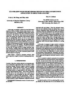
Fig. 3. Comparison of the noise reduction rates in (a) conventional MSICA1: FDICA is followed by NH-TDICA, (b) conventional MSICA2: FDICA is followed by NH-TDICA with spectral compensation, (c) conventional MSICA3: FDICA is followed by H-TDICA, (d) conventional MSICA4: FDICA is followed by H-TDICA with spectral compensation, and (e) proposed MSICA5: FDICA is followed by the proposed method combining H-TDICA and linear prediction. volved with the impulse responses specified by the reverberation times (RT) of 300 ms. The impulse responses are recorded in a variable reverberation time room. These sound data which are artificially convolved with the real impulse responses have the following advantages: (1) we can use the realistic mixture model of two sources and neglect the effect of background noise, (2) since the mixing condition is explicitly measured, we can easily calculate a reliable objective score to evaluate the separation performance as described in Sect. 5.3.

5. EXPERIMENTS AND RESULTS 5.1. Experimental Setup A two-element array with the interelement spacing of 4 cm is assumed. We determined this interelement spacing by considering that the spacing should be smaller than half of the minimum wavelength to avoid the spatial aliasing effect; it corresponds to 8.5/2 cm in 8 kHz sampling. The speech signals are assumed to arrive from two directions, −30◦ and 40◦ . The distance between the microphone array and the loudspeakers is 1.15 m. Two kinds of sentences, those spoken by two male and two female speakers are used as the original speech samples. The sampling frequency is 8 kHz and the length of speech is limited to within 3 seconds. Using these sentences, we obtain 12 combinations with respect to speakers and source directions. In these experiments, we use the following signals as the source signals: the original speech con-

5.2. Postprocessing for Spectral Compensation In order to compare the various ICAs fairly, we perform postprocessing for the spectral compensation of the separated signals in this experiment. This processing is based on the utilization of the inverse of the separation filter matrix for the normalization of gain

340

[3]. In this method, the following operation is performed: h i Y˜l (f ) = W (TD) (f )−1 [ 0, · · · , 0 , Yl (f ), 0, · · · , 0 ]T , (11) l

where Yl (f ) denotes the frequency-domain component of the lth estimated source signal by the TDICA part in MSICA, Y˜l (f ) denotes the l-th resultant separated source signal in the frequency domain after the spectral compensation ([·]l denotes the l-th element of the argument), and W (TD) (f ) is the frequency-domain representation of the separation filter matrix in the TDICA part, w(H) (τ ) or w(NH) (τ ). After the operation, we can obtain the spectrally compensated output signals in the time domain by applying the inverse DFT. In this experiment, we use the DFT and the inverse DFT of 218 points. By using W (TD) (f )−1 , the gain arbitrariness vanishes in the separation procedure. However, this procedure often fails and yields harmful results for signal reconstruction, particularly when the condition number of W (TD) (f ) is large because the invertibility of W (TD) (f ) cannot be guaranteed. 5.3. Objective Evaluation Score Noise reduction rate (NRR), defined as the output signal-to-noise ratio (SNR) in dB minus input SNR in dB, is used as the objective evaluation score in this experiment. The SNRs are calculated under the assumption that the speech signal of the undesired speaker is regarded as noise. The NRR is defined as NRR

≡

(O)

=

(I)

=

SNRl SNRl

(O)

2 1 X (O) (I) SNRl − SNRl , 2 l=1 P 2 f |Hll (f )Sl (f )| P , 10 log10 2 f |Hln (f )Sn (f )| P 2 f |All (f )Sl (f )| , 10 log10 P 2 f |Aln (f )Sn (f )|

(12)

(13) (14)

(I)

where SNRl and SNRl are the output SNR and the input SNR, respectively, and l 6= n. Also, Sl (f ) is the frequencydomain representation of the source signal, sl (t), Hij (f ) is the element in the i th row and the j th column of the matrix H (f ) = W (MSICA) (f )A(f ) where W (MSICA) (f ) denotes the entire separation process in MSICA including both FDICA and TDICA (even with the spectral compensation described in the previous section), and A(f ) is the mixing matrix which corresponds to the frequency-domain representation of the room impulse responses described in Sect. 2.

The length of the separation filters, w(H) (τ ) or w(NH) (τ ), is 2048. In the proposed algorithm, the order N in the linear predictor is 1024. Figures 3(a)–(e) show the NRR results of MSICA1–MSICA5 for different iteration points. These values were averages of all of the combinations with respect to speakers and source directions. The step-size parameters are chosen independently for each of the NH-TDICA, H-TDICA, and the proposed algorithm so that the NRR scores at the early iterations are almost the same in Figs. 3(a)– (e). From these results, the following are revealed. (1) In the conventional MSICA1 and MSICA2 in which the NH-TDICA is used, the behavior of the NRR is not monotonic and there are remarkably consistent deteriorations, even when the step-size parameter is changed. (2) In the proposed algorithm, MSICA5, there are no deteriorations of NRRs. Therefore, the separation performances are almost completely retained during all of the iterations. Regarding the separation performance of MSICA3 and MSICA4 in which the H-TDICA is used, the following are revealed. (1) The separation performance of MSICA3 is obviously superior to that of the proposed MSICA5. (2) However, its effective separation performance, i.e., the performance of MSICA4, is inferior to that of MSICA5. We speculate that the specious performance in MSICA3 is due to the exceeding emphasis of high-frequency components by the whitening effect of H-TDICA. Figure 4 shows the typical long-time averaged spectra of the separated signals obtained by MSICA3 and MSICA4. From these results, we can confirm the spectral distortion in MSICA3. In general, the separation in the high-frequency region is easier than that in low-frequency region [13, 14] because the reverberation is shorter as the frequency increases [15]. Thus, MSICA3 gains the improvement of the NRR only in the high-frequency region, and consequently we can conclude that MSICA3 is useless for separating the speech signals from the practical viewpoint. In order to confirm the convergence of each MSICA learning, we evaluate the frobenius norms of {·} parts on the right-hand side in Eqs. (4) and (9), which are defined as F N (NH)

=

F N (H)

=

Q−1 Q−1 1 X X T diag h ( y (t)) y (t − τ + d) i

t Q2 τ =0 d=0

−h(y (t))y (t − τ + d)T it , (15) Q−1 Q−1 1 X X

I δ(τ − d) Q2 τ =0

d=0

− h(v (t))v (t − τ + d)T it .

(16)

Figures 5(a) and (b) show F N (NH) of the conventional MSICA1 and F N (H) of the proposed MSICA5. These scores correspond to the stability of the iterative learning; it should be monotonically decreased. As shown in these figures, the conventional ICA loses its stability under the nonholonomic constraint. However, the proposed method can converge in every situation and consequently, we can conclude that the proposed algorithm is effective for improving the stability of the learning.

5.4. Experimental Results and Discussion In this study, we compare the following MSICAs: MSICA1: FDICA is followed by NH-TDICA, MSICA2: FDICA is followed by NH-TDICA with spectral compensation, MSICA3: FDICA is followed by H-TDICA,

6. CONCLUSION

MSICA4: FDICA is followed by H-TDICA with spectral compensation, and

We newly proposed a stable algorithm for BSS combining MSICA and linear prediction. In the proposed algorithm, the linear predictors estimated from the roughly separated signals by FDICA are

MSICA5: FDICA is followed by the proposed method combining H-TDICA and linear prediction.

341

-5

200

Power spectrum [dB]

-10 -15

(a) Conventional MSICA1

MSICA4

Frobenius Norm FN (NH)

Reference MSICA3

-20 -25 -30 -35

150

-6

α=2.0x10

-6

α=1.0x10

-7

α=5.0x10

100

50

-40 -45

0

500

0

1000 1500 2000 2500 3000 3500 4000 Frequency [Hz]

0

200


800

1000

16 Frobenius Norm FN (H)

Fig. 4. Comparison of the power spectra in conventional MSICA3: FDICA is followed by H-TDICA, conventional MSICA4: FDICA is followed by H-TDICA with spectral compensation, and reference signal (s1 (t) component recorded at the microphone). inserted before the holonomic TDICA as a prewhitening processing, and the dewhitening is performed after TDICA. The stability of the proposed algorithm can be guaranteed by the holonomic constraint, and the pre/dewhitening processing prevents the decorrelation. The experimental results under a reverberant condition revealed that the proposed algorithm results in the higher stability and higher separation performance, compared with the conventional MSICA including H-TDICA or NH-TDICA. Further study on the robustness against the background noise remains an open problem for the future.

14

(b) Proposed MSICA5

12 -4

α=1.0x10

10

-5

α=3.0x10

8

-5

α=1.0x10

6 4 2 0

0

200


800

1000

Fig. 5. Comparison of frobenius norms Eqs. (15), (16) in (a) conventional MSICA1: FDICA is followed by NH-TDICA and (b) proposed MSICA5: FDICA is followed by the proposed method combining H-TDICA and linear prediction.

7. ACKNOWLEDGEMENT The authors are grateful to Dr. Shoji Makino and Ms. Shoko Araki of NTT. CO., LTD for their greateful discussions. This work was partly supported by CREST (Core Research for Evolutional Science and Technology) of JST (Japan Science and Technology Corporation).

[8] S. Choi, S. Amari, A. Cichocki, and R. Liu, “Natural gradient learning with a nonholonomic constraint for blind deconvolution of multiple channels,” Proc. ICA99, pp.371–376, January 1999. [9] S. Araki, S. Makino, T. Nishikawa, and H. Saruwatari, “Fundamental limitation of frequency domain blind source separation for convolutive of speech,” Proc. ICASSP2001, pp.2737–2740, May 2001. [10] S. Kurita, H. Saruwatari, S. Kajita, K. Takeda, and F. Itakura, “Evaluation of blind signal separation method using directivity pattern under reverberant conditions,” Proc. ICASSP2000, pp.3140–3143, June 2000. [11] F. Asano, S. Ikeda, M. Ogawa, H. Asoh, and N. Kitawaki, “A combined approach of array processing and independent component analysis for blind separation of acoustic signals,” Proc. ICASSP2001, pp.2729–2732, May 2001. [12] A. Papoulis and S. U. Pillai, Probability, random variables and stochastic processes (Fourth Ed.), McGraw-Hill Series in Electrical and Computer Engineering, New York, 2002. [13] T. Nishikawa, T. Kawamura, H. Saruwatari, and K. Shikano, “Overdetermined source separation with blind beamformer,” The 2000 Autumn Meeting of the ASJ, pp.447–448, Sept. 2000 (in Japanese). [14] R. Aichner, S. Araki, S. Makino, T. Nishikawa, and H. Saruwatari, “Time domain ICA blind source separation of non-stationary convolved signals by utilizing geometric beamforming,” Proc. IEEE International Workshop on Neural Networks for Signal Processing, pp.445–454, Sept. 2002. [15] H. Kuttruff, Room acoustics (Fourth Ed.), Spon Press, London, 2000.

8. REFERENCES [1] P. Common, “Independent component analysis, a new concept?,” Signal Processing, vol.36, pp.287–314, 1994. [2] T. W. Lee, Independent component analysis, Kluwer academic publishers, 1998. [3] N. Murata and S. Ikeda, “An on-line algorithm for blind source separation on speech signals,” Proc. of 1998 International Symposium on Nonlinear Theory and Its Application (NOLTA98), pp.923–926, Sept. 1998. [4] L. Parra and C. Spence, “Convolutive blind separation of nonstationary sources,” IEEE Trans. Speech and Audio Processing, vol.8, no.3, pp.320–327, May 2000. [5] H. Saruwatari, T. Kawamura, and K. Shikano, “Blind source separation for speech based on fast-convergence algorithm with ICA and beamforming,” Proc. Eurospeech2001, pp. 2603–2606, Sept. 2001. [6] S. Amari, S. C. Douglas, A. Cichocki, and H. H. Yang, “Multichannel blind deconvolution and equalization using the natural gradient,” Proc. SPAWC97, pp.101–104, April 1997. [7] T. Nishikawa, H. Saruwatari, and K. Shikano, “Comparison of timedomain ICA, frequency-domain ICA and multistage ICA,” Proc. EUSIPCO2002, vol.II, pp.15–18, Sept. 2002.

342