AbstractâIn this paper, we propose to introduce the bootstrap resampling technique in the generalized mixture estimation. The generalized aspect comes from ...
Introduction of the bootstrap resampling in the generalized mixture estimation Ahlem Bougarradh, Slim M’hiri and Faouzi Ghorbel CRISTAL Laboratory, GRIFT Research Group National School of Computer Sciences University of Manouba, 2010 Tunisia
Abstract—In this paper, we propose to introduce the bootstrap resampling technique in the generalized mixture estimation. The generalized aspect comes from the use of the probability density function (pdf) estimation coming from the Pearson system. The bootstrap sample is constructed by randomly selecting a small representative set of pixels from the original image. The application of the Bootstrapped Generalized Mixture Expectation Maximization algorithm BGMEM led us to define a new empirical criterion of representativity of the sample. We give some simulation results for the determination of the empirical criterion. We validate our criterion by the application of the algorithm to the problem of unsupervised image classification.
I. I NTRODUCTION In statistical segmentation[4], [5], [14], [15], the image is considered as a realization of mixture distributions [13]. The estimation is an essential step for the estimation of the mixture distribution parameters. It can be achieved by the ExpectationMaximization (EM) algorithm which was proposed in [2], [7] for parametric unsupervised Bayesian classification. It is an iterative procedure, which assumes that the mixture probability density function of data is a linear combination of a finite number of gaussian distributions where the coefficients of this combination are the a priori probability of each class. Using the Pearson system [10], [6], a generalized mixture segmentation can be realized by the GMEM algorithm [6]. The Pearson system is a finite family of distributions including gaussian, gamma, beta, inverted beta. The different distribution shapes provided by this system improve the estimation of non symmetric histogram which characterizes radar [11] and ultrasound images. Effectively, the mixture identification by the GMEM consists of to the estimation of the high order moments of the conditional probability density function of each class compared to the Gaussian EM. During iterations, two parameters called ’skewness’ and ’kurtosis’ are computed. The parameters are needed in the decision rule of Pearson system witch consist on selecting in this system the appropriate conditional pdf for each class. In statistical segmentation, the time increases with the size of training data set. In most of the real-world applications, the size of the training data is very large. As a result, the time required to segmentation could be prohibitively large. This pragmatic constraint calls for data reduction, which means selecting an appropriate subset of the original training data set without reducing the segmentation accuracy significantly. Bootstrapping is a method
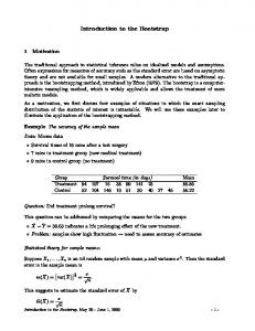
of mapping or re-sampling the given data. In statistics, it has been used for re-sampling [8]. Ghorbel [9] proposed to apply the bootstrap technique in image segmentation. The EM family of algorithms methods is improved by adding an optimal Bootstrap sample selection and decorrelation step to the blind approach. Criteria of representativity of the bootstrap sample are defined in [9]. They are recently extended to the global case [12]. By this technique, the parameter estimation would be made with the only use of a small number of representative samples instead of all the correlated pixels in the real image. In this paper, we propose to apply the bootstrap sampling to the GMEM algorithm. Some simulations will be studied showing the efficiently of the proposed representative criterion of the sample in bootstrap generalized mixture identification. The mean integrated square error is computed for the simulation study. The paper is organized as follows: in Section II, we describe the generalized mixture expectation maximization algorithm GMEM. Section III is devoted to the presentation of the proposed bootstrap generalized expectation maximization algorithm BGMEM. In Section IV the BGMEM is applied on a synthetic image for showing the efficiently of the representative criterion. In Section V we conclude from the ideas discussed throughout the paper. II. G ENERALIZED MIXTURE IDENTIFICATION A. Pearson system of distributions The Pearson system consists of a set of height families of distributions, including Gaussian, Gamma and Beta ones. Comprehensive introduction and detailed statements on the Pearson’s system are given in [10]. All the families parameters can be expressed in terms of the mean, variance, skewness and kurtosis, which leads to very flexible distribution forms. All the distributions can be represented in the Pearson’s graph (Figure1). Gaussian distributions are located at (β1 = 0, β2 = 3), Gamma distributions on the straight line β2 = 1.5β1 + 3 and inverse Gamma distributions on the curve with the equation 3 3 (−13β1 −16−2(β1 +4) 2 ). First kind Beta distribβ2 = β1 −32 utions are located between the lower limit and the Gamma line, second kind Beta distributions are located between the Gamma and the inverse Gamma distributions, and Type 4 distributions are located between the inverse Gamma distributions and the upper limit. Then, it is possible to estimate the empirical
A. Description of the BGMEM algorithm
1 Symmetric beta 2
3
Lower limit Gaussian Beta first kind
β2
4 Type7
Inverted Gamma
5
Gamma
6
inverted beta Upper limit Type 4
7
8
0
0.5
1
β
1.5
2
2.5
1
Fig. 1.
Pearson system graph
moments of a distribution from a sample, assess to its family of distributions from coordinates (β1 , β2 ), and determinate the parameters that precisely characterize the probability density function [6]. B. The generalized mixture expectation maximization algorithm The classical EM algorithm based on Gaussian distribution is generalized to the use of all distributions coming from the Pearson system and so, the generalized mixture expectation maximization GMEM algorithm [6] will be more adapted to fit non symmetric histogram. The GMEM algorithm follows the steps of the classical EM algorithm, it assumes that the observed image is a realization of a generalized mixture distribution, so that the function (pdf) is �Kprobability density� K written as f (y, θ) = j=1 f (y, θj )πj with j=1 πj = 1 and πj � 0 for each class j. f (y, θj ) is the conditional pdf coming from the Pearson system and πj is the prior probability of a class j. The particularity of this algorithm resides on the estimation of the third and fourth order moments needed in the computation of the skewness and kurtosis. The GMEM algorithm present a detection law step in witch the appropriate conditional distribution is selected for each class.
The BGMEM algorithm is iterative, it consists on iterating the GMEM algorithm B times. In each iteration, a bootstrap sample is selected and the parameters estimation are done under the sample not on the whole image. In each bootstrap iteration, the parameters estimation of the sample follow the four following steps: • Initialization Step : – Case B = 1: For all the classes of the mixture, the laws are Gaussian, the proportion is taken equally, the means are calculated by a kmeans algorithm and the variances are taken the same , They are chosen equal to maximum the grey level of the image. – Case B � 2: The parameters of the bootstrap sample are initialized by those estimated on the previous sample. • Selection law step: in this step, the appropriate conditional distribution from the Pearson system will be selected for each class. The Pearson rule of the selection law is given in [6]. • Expectation Step: consists on the estimation of the posterior probability for a pixel belonging to the class k at the iteration q. πkq−1 fk (yi |θk ) K � q−1 πl fl (y1 |θlq−1 )
(1)
l=1
•
Maximization Step: the parameters of the mixture are constructed in the following way: N � (q) πk
∀k ∈ {1, ..., K}
=
(q)
∀k ∈ {1, ..., K}
µ1,k =
P (xk |yi , θq )
i=1
(2)
N N �
III. T HE PROPOSED BOOTSTRAPPED GENERALIZED
P (xk |yi , θq )yi
i=1 N �
(3) q
P (xk |yi , θ )
i=1
MIXTURE IDENTIFICATION
The bootstrap resampling consists on selecting a random sample from an image. The application of this technique in image segmentation has shown two principles advantages. The first consists on the decorrelation of the pixels in the sample and the second in the reduction of the time computing. Some works [9],[12] are done in order to determine the optimal minimum representative set of pixels from the original data. The size of the bootstrap sample is defined according to a representative criteria introduced in the blind Gaussian mixture case [9] and extended to the global Gaussian mixture case [12]. We propose in this section to use the bootstrap resampling technique with the generalized mixture expectation maximization algorithm.
(q−1)
(q)
Pik =
∀k ∈ {1, ..., K}
N � (q)
∀k ∈ {1, ..., K}µ2,k =
i=1
(q)
(q)
P (xk |yi , θq )(yi − µ1,k )(yi − µ1,k ) N �
P (xk |yi , θq )
i=1
N � (q)
∀k ∈ {1, ..., K} µ3,k =
i=1
(4) (q)
P (xk |yi , θq )(yi − µ1,k )3 N � i=1
(5) q
P (xk |yi , θ )
0.012
N �
∀k ∈ {1, ..., K}
(q) µ4,k
=
q
P (xk |yi , θ )(yi −
i=1 N �
original densities
0.01
(q) µ1,k )4
0.008
(6) P (xk |yi , θq )
0.006
i=1 0.004
At the q t h iteration on the sample the skewness and the kurtosis of the class k are computed as: (q) β1,k
(q)
0.002
(q) 2
=
β2,k =
(µ3,k )
(q) 3 (µ2,k )
µ4,k
(q) 2 (µ2,k )
0
0
50
100
150
200
250
(7) Fig. 2.
(8)
Mixture to identify
0.012
0.012
original densities f1π1
0.01
original densities f1π1
0.01
f2π2
f2π2
fπ
fπ
3 3
The algorithm applied to the sample stops when the sample parameters are stagnated. The end of the BGMEM algorithm (when B=25) [12] gives the final estimated parameters. Being in the blind case, the size of the bootstrap sample is taken according to the representative criterion given in [9]. So, the optimal size of the sample is mentioned equal to 4K where K is the dynamic of the image. B. Simulation In this section, we propose in a first time to generate a mixture of two beta law and to estimate in a second time the parameters of the mixture by a variety of EM algorithm. From Pearson system a beta law is written: (y−b1 )p−1 (b2 −y)q−1 1 for y ∈ [b1 , b2 ]; B(p,q) p+q−1 , (b2 − b1 ) f (y) = 0 otherwise. (9) The parameters p, q, b1 and b2 of this distribution are computed from some equations given in [6] knowing the mean,variance,skewness and kurtosis of the sample. The densities generated are shown in the figure2 bellow. The estimation is done in the classical case by the gaussian EM algorithm which shows the inadequate use of the gaussian law in the case of non symmetric histogram (Figure 3(a)). The application of the GMEM algorithm yields a good quality of estimation(Figure 3(b)) Fixing the size of the sample to 4K where K is the dynamic of the mixture as representativity criterion for the gaussian mixture, we randomly select a set of pixels with the size 4K and then we estimate the parameters of the mixture by the BGMEM algorithm. Fig4 shows the fitting of the estimated conditional densities by the BGMEM to the theoretical ones. The quality of estimation is worse than the one obtained by the GMEM. We conclude that the size of the sample is not enough large to preserve a good quality of estimation.
3 3
f1π1+f2π2+f3π3
0.008
0.006
0.006
0.004
0.004
0.002
0.002
0
0
50
100
150
200
f1π1+f2π2+f3π3
0.008
250
0
0
50
100
(a)
150
200
250
(b)
Fig. 3. (a) Identification by the gaussian algorithm, (b) identification by the generalized mixture algorithm
C. Empirical representative criterion for BGMEM We propose an experimental study to find the appropriate size of the sample. We proceed by increasing the bootstrap sample of generated data presented in section III-B proportionally to K from 4K to 20K, applying the BGMEM on the sample and computing the Mean Integrated Square Error (MISE). The curve of the Figure 5 presents two variations. The first is a decreasing variate which indicates that more the sample is large, better the quality of estimation will be. The second 0.014
original densities f1π1
0.012
fπ
2 2
fπ
3 3
0.01
f π +f π +f π 1 1
2 2
3 3
0.008
0.006
0.004
0.002
0
0
50
100
150
200
250
Fig. 4. Identification by the bootstrap generalized mixture algorithm with the size 4K of the sample
−3
5
x 10
0.03
4.5
MISE
original densities
0.025
4
0.02
3.5
3
0.015
2.5
0.01 2
0.005
1.5
1
0.5
0 20 4
5
6
7
8
9
10
11
12
13
30
Fig. 5. Evaluation of the Mean Integrated Square Error MISE for different sizes of sample, the size is taken equal to n*k where n is an integer greater than 4 and K is the grey level variation
0.012
50
60
70
80
90
100
Fig. 7.
Pearson system graph
0.012
original densities fπ
original densities fπ
1 1
0.01
1 1
0.01
f2π2
f2π2
f3π3
f3π3
f1π1+f2π2+f3π3
0.008
0.006
0.004
0.004
0.002
0.002
0
50
100
150
200
f1π1+f2π2+f3π3
0.008
0.006
0
40
14
250
0
0
50
(a)
100
150
200
250
(b) (a)
Fig. 6. Identification of the mixture by the bootstrap generalized algorithm switching the size of the sample:(a) size=11K, (b) size=20K
is a constant variate which shows that under a fixed size of sample, the quality does not change and the MISE is almost stagnated. We show in the figure6 the estimated conditionals density from two samples with sizes 11K and 20K where K is the dynamic of the grey level of the sample. The figure shows a same quality of fitting theoretical densities. This fact confirms that under a fixed size of sample, we obtain a same quality of estimation. This size made the sample representative. We are done many simulations with different classes and different grey level for testing the criterion. We can conclude that a size of 11K preserves a good quality of estimation and it will be presented as an empirical representative criterion for the BGMEM algorithm.
Fig. 8.
(a) A binary image, (b) the noised image
N umber of misclassif ication pixels T otal number of pixels
τ=
(10)
We propose to estimate the conditional densities for each class of the mixture by the BGMEM algorithm with the size 4K and 11K of the sample then by the GMEM algorithm. Fig.9 confirms the insufficiency of the size 4K of the sample, the estimated densities doesn’t fit the theoretical . This size of the sample must be greater than 11K to preserve good results in parameter estimation (Figure 10).For this size,
0.03
original densities fπ
0.025
IV. VALIDATION ON UNSUPERVISED BAYESIAN
1 1
f2π2
CLASSIFICATION
In this section, we propose to validate the BGMEM algorithm on the unsupervised image classification. We generate a synthetic image showed in figure8(b) by noising a binary image with the noise intensity (Figure 7) belonging to the Pearson system. The size of the binary and synthetic images is 128*128, they are composed of two classes with the proportion of grey level is 1/3 and 2/3. The use of synthetic image provides us the calculus of the error rate classification which is defined as:
(b)
f1π1+f2π2
0.02
0.015
0.01
0.005
0 20
Fig. 9.
30
40
50
60
70
80
90
100
Mixture parameters identification by the BGMEM with the size 4k
0.03
original densities fπ
0.025
1 1
fπ
2 2
f π +f π
0.02
1 1
2 2
0.015
0.01
0.005
0 20
30
40
50
60
70
80
90
100
(a)
(b)
Fig. 10. Mixture parameters identification by the BGMEM with the size 11k Fig. 12. Image classification using:(a) GMEM algorithm, (b) BGMEM algorithm with the size 11K of the sample 0.03
original densities f1π1
0.025
use of the gaussian law for non symmetrical histograms. Fig12 shows a same quality of image classification using the GMEM algorithm on the whole image and the BGMEM with a size 11K of the sample.
fπ
2 2
f π +f π
0.02
1 1
2 2
0.015
0.01
V. C ONCLUSION 0.005
0 20
Fig. 11.
30
40
50
60
70
80
90
100
Mixture parameters identification by the GMEM
both the classical GMEM and the BGMEM present the same quality of estimation for the different mixture (Figure 11). In unsupervised image classification, in addition of the problem of estimation, we can evaluate a quality of classification by computing the error rate of classification witch gives a percentage of the misclassification pixels in the image. The evaluation of the error of classification of the synthetic images is given in Table I. The results obtained in Table I confirms that the size 4K of the sample isn’t appropriate to do the classification by the BGMEM algorithm because it presents an error rate greater than the one obtained with GMEM. The quality of classification of the BGMEM for the size 11K of the sample is better than the one obtained with the GMEM algorithm. This result comes from the fact that the bootstrap technique eliminates the correlation between the pixels on the image and then offers a best condition of the application of the EM algorithm which is based on maximization of the likelihood. For this noise, the error rate classification obtained by the gaussian EM is the greatest. This fact confirms the inadequacy Error Noise
Gaussian GM EM 0.3921 0.3098
BGM EM 4K BGM EM 11K 0.3189 0.3093
TABLE I T HE ERROR RATE CLASSIFICATION OF THE SYNTHETIC IMAGE .
The application of the bootstrap technique for the generalized mixture identification has allowed us to define a new algorithm called BGMEM. This method of estimation has led us to define by simulations an empiric criterion of representativity of the sample, since the theoretical study of the criterion is difficult. To define this criterion, the MISE is calculated under different size of samples and the point fixed correspond to the optimal size of the sample witch guaranties a good quality of estimation and is small enough for reduction of the time computing. The application of the proposed BGMEM algorithm to the problem of unsupervised Bayesian image classification allows to have good quality of classification and so to filter the non symmetric noise. Our future works in the mean will consider the extension of the statistical model to the multivariate case. Such extensions have advantage in the mean of the consideration of the contextual information in the segmentation procedure. However; it assumes that we can define the multivariate Pearson system. R EFERENCES [1] H. Kopka and P. W. Daly, A Guide to LATEX, 3rd ed. Harlow, England: Addison-Wesley, 1999. [2] Ambroise C. and Govaert G., Convergence of an EM-type algorithm for spatial clustering. Pattern Recognit. Lett. 19 (1998), pp. 919-927. [3] Banga C. and Ghorbel F. ; Optimal Bootstrap Sampling for Fast Image Segmentation : Application to Retina Image, IEEE International Conference on Acoustics, Speech, and Signal Processing, Minneapolis, USA, Vol. 5, pp.638 641, 1993. [4] Caillol H., Pieczynski W. and Hillion A., Estimation of fuzzy Gaussian mixture and unsupervised statistical image segmentation. IEEE Trans. Image Process. 6 (1997), pp. 425-440. [5] Chalmond B., An iterative Gibbsian technique for reconstruction of m-ary images. Pattern Recognit. 22 (1989), pp. 747-761. [6] Delignon Y., Marzouki A., et Pieczynski W. ; Estimation of Generalised Mixture and Its Application in Image Segmentation, IEEE Transactions on Image Processing, Vol. 6, N 10, pp. 1364 1375, 1997.
[7] Dempster A., Laird N. et Rubin D. ; Maximum Likelihood from Incomplete Data via the EM Algorithm. Journal of Royal Statistical Society, Series B, Vol. 39, pp. 1 38, 1977. [8] Efron B. ; Bootstrap Method : Another Look at the Jackknife, Annals of Statistics, Vol. 7, pp. 1 26, 1979. [9] Ghorbel F. and Banga C. ; Bootstrap sampling applied to image analysis, invited paper, special session, IEEE-ICASSP, Adelaide, South Australia, Vol. 6, pp. VI 81-84, 1994. [10] Johnson N.L. and Kotz S. , Distribution in statistics: Continuous univariate distribution, Wiley-interscience, 1969. [11] Masson P. and Pieczynski W., SEM algorithm and unsupervised statistical segmentation of satellite images. IEEE Trans. Geos. Rem. Sen. 31 (1993), pp. 618-633. [12] Mhiri S, Cammoun L. et Ghorbel F., Speeding up HMRF EM algorithms for fast unsupervised image segmentation by Bootstrap resampling: Application to the brain tissue segmentation. J. Signal Processing 87 (2007),pp 2544-2559. [13] Pieczynski W., Estimation of context in random field. J. Appl. Stat. 16 (1989), pp. 283-290. [14] Zhang Y.J., Evaluation and comparison of different segmentation algorithms. Pattern Recognit. Lett. 18 (1997), pp. 963-974. [15] Zribi M. and Ghorbel F., An unsupervised and non-parametric bayesian classifier. Pattern Recognit. Lett. 24 (2003), pp. 97-112.