Comparison of Bootstrap Resampling Methods for 3-D PET Imaging

1442

IEEE TRANSACTIONS ON MEDICAL IMAGING, VOL. 29, NO. 7, JULY 2010

Comparison of Bootstrap Resampling Methods for 3-D PET Imaging C. Lartizien*, J.-B. Aubin, and I. Buvat

Abstract—Two groups of bootstrap methods have been proposed to estimate the statistical properties of positron emission tomography (PET) images by generating multiple statistically equivalent data sets from few data samples. The first group generates resampled data based on a parametric approach assuming that data from which resampling is performed follows a Poisson distribution while the second group consists of nonparametric approaches. These methods either require a unique original sample or a series of statistically equivalent data that can be list-mode files or sinograms. Previous reports regarding these bootstrap approaches suggest different results. This work compares the accuracy of three of these bootstrap methods for 3-D PET imaging based on simulated data. Two methods are based on a unique file, namely a listmode based nonparametric (LMNP) method and a sinogram based parametric (SP) method. The third method is a sinogram-based nonparametric (SNP) method. Another original method (extended LMNP) was also investigated, which is an extension of the LMNP methods based on deriving a resampled list-mode file by drawings events from multiple original list-mode files. Our comparison is based on the analysis of the statistical moments estimated on the repeated and resampled data. This includes the probability density function and the moments of order 1 and 2. Results show that the two methods based on multiple original data (SNP and extended LMNP) are the only methods that correctly estimate the statistical parameters. Performances of the LMNP and SP methods are variable. Simulated data used in this study were characterized by a high noise level. Differences among the tested strategies might be reduced with clinical data sets with lower noise. Index Terms—Bootstrap, noise properties, positron emission tomography (PET).

I. INTRODUCTION

C

HARACTERIZING the noise properties of positron emission tomography (PET) images based on a unique scan or a small number of repeated samples is highly desirable in clinical practice to estimate the errors affecting measurements made from the images. This would also facilitate the use of model observers for estimation and detection tasks [1]. Analytical derivations of the variance have been proposed for

Manuscript received November 25, 2009; revised March 05, 2010; accepted March 10, 2010. First published April 19, 2010; current version published June 30, 2010. Asterisk indicates corresponding author. *C. Lartizien is with the CREATIS, CNRS UMR 5220, INSERM U630, INSA-Lyon, Lyon University, 69621 Lyon, France (e-mail: carole. [email protected]). J.-B. Aubin is with the Laboratoire de Mathématiques Appliquées de Compiègne (LMAC), Université Technologique de Compiègne, 91406 Compiègne, France (e-mail: [email protected]). I. Buvat is with the CNRS UMR 8165—Paris 7 University—Paris 11 University, 60205 Orsay, France (e-mail: [email protected]). Digital Object Identifier 10.1109/TMI.2010.2048119

images reconstructed from the filtered back projection (FBP) [2], [3] and the maximum-likelihood expectation-maximization (MLEM) [4]–[6] algorithms but they require approximations, the most critical of which being that the recorded counts in the projection are Poisson distributed. Although PET emission process is described by a Poisson statistic, many processing steps of the raw signal change the voxel values to non-Poisson variates. Bootstrap resampling methods [7] have been proposed as an alternate to analytical methods to estimate the statistical properties of PET and single photon emission computed tomography (SPECT) images [8]–[12]. The bootstrap approach consists in generating multiple statistically equivalent data sets from few samples of data, i.e., data sets that are samples from the same multivariate probability distribution as the original data. A first group of bootstrap methods in PET and SPECT [8], [10] is based on a parametric approach which assumes that data from which resampling is performed follows a Poisson distribution [8]. The original data is a unique sinogram or a unique list-mode file. Bootstrap replicates (sinograms or list mode files) are then produced by estimating the parameter of the Poisson distribution from the original file. For the sinogram-based method, this means that each bin of a bootstrap sinogram is randomly drawn from a Poisson distribution whose parameter is the corresponding bin value of the original file. An alternative solution is to consider a few sets of statistically equivalent original data instead of a unique sample to better estimate the parameter of the Poisson distribution. A second group of methods is based on nonparametric approaches [9], [11]. A method based on a unique list-mode file consists in randomly choosing events from this file with replacement to produce a number of new list-mode files of the same size as the original file [10]. Another method uses a set of statistically equivalent sinograms [9], [11]. Bootstrap sinograms are then produced by randomly choosing sinogram bins from the set of original sinograms. Haynor and Woods [8] produced resampled list-mode and sinogram PET data sets from one original file using the parametric bootstrap approach assuming a Poisson distribution. They showed that this method allowed an accurate estimate of the variance in the final reconstructed image. More recently, Dahlbom [10] generated list-mode data files from one original 2-D list-mode ECAT HR PET data set by choosing events at random and with replacement. Considering different reconstruction algorithms, he showed that the standard deviation images derived from the bootstrap list-mode files closely agreed with the standard deviation images derived from repeated scans. D’Asseler et al. [12] used the same nonparametric bootstrap method as Dahlbom for 2-D simulated PET data and found

0278-0062/$26.00 © 2010 IEEE

LARTIZIEN et al.: COMPARISON OF BOOTSTRAP RESAMPLING METHODS FOR 3-D PET IMAGING

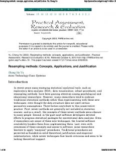
that the mean background of the bootstrap realizations and the mean background of the noisy realizations were different. Kim et al. [11] used a non-parametric sinogram-based bootstrap technique for precorrected 2-D GE Advance PET data in which each distance-angle bin of the resampled sinogram was uniformly drawn from subsets of experimental and statistically equivalent sinograms. They found equivalent mean values between images reconstructed from the resampled data and from repeated acquisitions, but some discrepancies in variance values. Finally, Buvat [9] generated resampled data by randomly choosing one row (instead of one bin) from a set of statistically equivalent original sinograms, in order to potentially account for noise correlation within a row. This nonparametric method was shown to produce accurate estimation of moments of order 1–3 and of the 1-D local covariance on simulated SPECT and real 2-D PET data. This short review suggests that bootstrap methods might be used for the estimation of 3-D PET statistical properties, but underlines some contradictory results. This work aims at comparing three bootstrap methods in the context of 3-D PET, namely the list-mode based nonparametric (LMNP) method used by Dahlbom [10], the sinogram-based parametric (SP) method proposed by Haynor and Woods [8], and the sinogram-based nonparametric (SNP) method by Buvat [9]. Another original method was also investigated which is an extension of the LMNP methods based on deriving a resampled list-mode file by drawing events from multiple original list-mode files. The main purpose of this study is to compare different bootstrap methods and derive guidelines regarding their use for 3-D PET imaging as a function of the type (list mode or sinograms) and statistics of the original data set. A question we address in this study is whether we can generate accurate resampled PET data series, each of a fixed number of events, from a unique list-mode file or a unique sinogram of events. A positive answer to this of the same number question would open new perspective for the development of patient-specific statistical image processing methods. This study used simulated data obtained with the GATE Monte Carlo simulation tool [13] for a scanner geometry equivalent to the MicroPET R4 manufactured by Siemens Preclinical Solutions [14]. II. MATERIALS AND METHODS A. 3-D PET Data Monte Carlo Simulations The GATE Monte Carlo simulation tool used in this study can model most of the phenomena encountered in PET acquisitions including scattered and random components of the PET signal, dead-time effects and contamination from activity outside the field-of-view [13]. This tool has already been validated for different PET and SPECT scanner geometries. 3-D PET data were simulated for a scanner geometry equivalent to that of the small animal MicroPET R4 scanner [14]. The axial and transverse fields-of-view of this scanner are 78 and 91 mm, respectively. The phantom geometry shown in Fig. 1 consisted of three 2-cm-diameter water cylinders of uniform activities located in an 8-cm-diameter water cylinder. The ratios between the small cylinder activity and the background activity

1443

Fig. 1. 3-D view of the simulated object. Activity ratios with respect to the background were 10:1, 15:1, and 20:1.

were 10:1, 15:1 and 20:1, respectively. All cylinders were 2 cm long and the activity in the 8-cm-diameter cylinder was 4 MBq. The acquisition time was set to 5 s which corresponded to approximately 1.88 million detected coincidence events. B. Bootstrap Resampling Five hundred and fifty-one statistically equivalent list-mode files (each containing about 1.88 million detected coincidences) were generated with GATE using the LMF list-mode format proposed by the Crystal Clear Collaboration [15]. Five hundred repeated scans were used as a gold standard and are referred to as GS in the following. The remaining 51 statistically equivalent samples were used to generate five series of 500 bootstrap resampled data as follows. • One of the list-mode files was used to derive 500 resampled list-mode files based on the nonparametric method proposed by Haynor and Woods [8] and used by Dahlbom [10]. Each resampled list-mode file contains the same number of events as the original file. In this technique, events are chosen at random and with replacement among the original list-mode events. One event from the original file may thus be selected more than once in a bootstrap data set. This method is referred to as LMNP in the following. • The same list-mode file was first rearranged into 3-D sinograms using a program described in Section II-C. This sinogram was then used to derive 500 resampled 3-D PET sinograms based on the parametric bootstrap approach proposed by Haynor and Woods that consists in drawing each bin of the resampled sinogram from a Poisson distribution with parameter equal to the corresponding bin value in the original sinogram. This method is referred to as SP in the following. • Fifty of the original list-mode files were rearranged into 3-D sinograms. Two series of 500 resampled sinograms each were then sampled from two original sets of 10 and 50 of these sinograms respectively using the method proposed by Buvat. This method consists in randomly choosing each rows row of a bootstrap sinogram among the corresponding to the same projection angle in the original sinograms. These data series are referred respectively to as SNP10 and SNP50 in the following. The 10 and 50 parameters were chosen to assess the impact of the number of original sinograms the SNP bootstrap approach is performed from. • The same series of 50 original list-mode files as the ones used in the SNP method were used to derive 500 resampled list-mode files following a non-parametric method derived

1444

from the LMNP method described above. For each resampled LM file, each event was drawn from the original data series by first choosing at random one of the 50 files and then choosing one event at random and with replacement in this selected file. The total number of events of each resampled file was chosen at random among the values of the 50 original files (close to 1.88 M detected coincidences). This method is referred to as LMNP50 in the following. The LMNP and SP methods are two methods based on a unique original sample and they produce bootstrap replicates of the same statistics as that of the original sample. The other three methods (SNP10, SNP50, and LMNP50) are based on a set of statistically equivalent original samples and produce replicates of the same statistics as that of one of the original sample. While the main objective of this study was to evaluate and compare the statistical properties of the images obtained from the resampled sinograms, some elements of statistical analysis of the resampled sinogram properties are presented in Appendix I for the LMNP, SP, and SNP methods. This analysis is intended to provide some insight into the statistical meaning of the bootstrap approaches. C. Data Reconstruction List mode data were rearranged into 3-D and 2-D sinograms using a rebinning program based on the library proposed by the Crystal Clear Collaboration to handle the LMF list-mode data format. This program identifies each couple of crystals corresponding to any given line of response of the LMF coincidence file and increments the bin of the corresponding sinogram based on a precomputed lookup table. The corresponding sinograms are thus not corrected for arc effects. The 3-D data were rearranged with a span of 1 and a maximum ring difference (mrd) of 10. The number of segments after rebinning was 21 and the number of coincidence events was about 7.5 10 . The 2-D sinograms were rearranged with a span of 1 and an mrd of 1. The number of segments after rebinning was 3 and the number of coincidence events was about 1.1 10 . The raw data, i.e., without any correction for attenuation, scatter, random, or geometrical effects were reconstructed using the STIR library [16]. The 3-D sinograms were reconstructed using the 3-D implementation of the FBP algorithm referred to as FBP3D in the following with a ramp filter and a cutoff frequency of 0.5 voxel . The 2-D sinograms were reconstructed with the ordered subset expectation maximization algorithm (OSEM2D) using four subsets and 16 iterations. Parameters of the FBP and OSEM reconstructions were set as the standard values recommended by the microPET R4 manufacturer for preclinical imaging [17]. This resulted in reconstructed images with dimensions 87 87 63 and an isotropic voxel size of 1.2115 mm . D. Statistical Properties of the Resampled Images The statistical properties of the reconstructed images were characterized for the five series of bootstrap resampled data (LMNP, SP, SNP10, SNP50, and LMNP50) and for each reconstruction scheme (FBP3D, OSEM2D). They were compared with the same statistical properties measured on the reference GS series of statistically equivalent samples. These properties included 1) the estimated point probability density function


(PDF), 2) the moment of order 1 (mean) and of order 2 (variance) images, and 3) the 1-D local covariance. Comparison of the mean and variance images included a statistical analysis based on the nonzero voxels of a reconstructed transverse image of the cylindrical phantom (See Fig. 4 for an illustration of such an image). For this study, was equal to 5261 voxels. For the data series to accurately describe the population statistical parameters, the number of samples should exvoxels. One way to achieve this ceed the number of simfor the GS data series would be to generate at least ulated replicates which would be very time consuming. Indeed, the generation of one 3-D LMF file was around 16 h on a standard PC running Linux and the size of one original single event list-mode file was around 253 Mb. We chose instead to consider the 12 central reconstructed planes of each of the 500 image replicated “samples.” volumes, resulting in These 12 adjacent axial planes all cross the cylindrical phantom and are reconstructed from the same number of original lines of responses (LORs). Each of these LORs only contributes to one specific plane so that there is no axial correlation between these planes. 1) Probability Density Function: We first compared the point probability density function (PDF) of the GS and bootstrap images by calculating the distribution of single voxel values over the entire set of data. This voxel was chosen at the center of the hottest cylinder of Fig. 1. The estimated PDF were obtained using 6000 voxels values each (1 voxel/plane 12 planes 500 replicates). 2) Estimated Mean and Variance Images: The moment of , was computed as order 1 or mean images, (1) is the value of voxel in the th sample of the where reconstructed images. The moment of order 2 or variance images was also computed as the diagonal elements of the covariance matrix M2 defined as

(2) The mean and variance images were computed for 10, 500, and 6000 samples in order to estimate the convergence speed of the statistical metrics of interest. The comparison of the GS and bootstrap mean and variance images was based on a visual analysis followed by a quantitative analysis using two error measures described in Wilson et al. [18] and Soares et al. [19]. The first error measure is the root mean square (rms) per cent error defined as (3) where stat can either represent the variance or the mean, is the estimated statistic in voxel of the GS images and


1445

Fig. 2. Histograms of a voxel centered on the hottest cylinder of the reference and resampled images reconstructed with FBP3D. These distributions were obtained using 6000 replicate images.

is the corresponding value in the images derived from the bootstrap data. The second error measure is the average percent bias defined as (4) The rms and bias were calculated in a 9 9 voxel region-ofinterest centered in the hottest cylinder of the mean and variance images derived from 6000 samples. A nonparametric Friedman analysis of variance [20] was performed on the six mean images estimated from the 6000 samples of the reference data and from the 6000 samples of each of the five resampled data series. This analysis tested the null hypothesis that these six populations of samples were drawn from the same population (see Appendix II). A similar analysis was conducted on the variance images. When the Friedman analysis demonstrated a global significant difference among the different methods, a post-hoc test for multiple comparisons was performed using the method of the smallest significant difference (SDD) [20] to determine which methods differed (see Appendix III). A nonparametric global test for variance homogeneity among the six methods was performed on the mean and variance images using the Box’s M test [20] (see Appendix IV). All statistical tests were applied on all nonzero voxels of the 12 central reconstructed planes of the 3-D and 2-D PET image volumes.

3) 1-D Local Covariance: Finally, we compared the 1-D local covariance at a specific image position obtained by plotfor the ting the elements of the covariance matrix voxel value and a correlation distance of voxels in the direction. Voxel was chosen in the background activity of the cylinder. The estimated 1-D local covariance plots were obtained using the 6000 replicate values of voxel . III. RESULTS A. Estimated Probability Density Function (PDF) Fig. 2 shows the distributions of values for a single image voxel in the background of the cylinder shown in Fig. 1. These histograms were obtained using 6000 replicates of the reference and resampled images reconstructed with FBP3D. Fig. 3 shows similar results for images reconstructed with OSEM2D, respectively. Fig. 2(c), (d), (e) and Fig. 3(c), (d), (e) show a good agreement between the histograms of the GS images and of the resampled images generated from the three bootstrap methods based on multiple original data, namely SNP10, SNP50, and LMNP50. The histograms corresponding to the bootstrap methods based on a unique file (LMNP, SP) were similar but did not match well the gold standard histogram [Fig. 2(a), (b), Fig. 3(a), (b)]. B. Comparison of the Mean Images Fig. 4 shows the mean transverse images of the 3-D image volumes reconstructed with FBP3D and averaged over 10 (column 1), 500 (column 2), and 6000 (column 3) replicates.

1446


Fig. 3. Histograms of a voxel centered on the hottest cylinder of the reference and resampled images reconstructed with OSEM2D. These distributions were obtained using 6000 replicate images.

The first row (row a) corresponds to the reference mean images computed from the repeated scans and the other rows (rows b–f) correspond to the mean images derived from the five series of resampled data. These images are displayed with the same intensity range of the gray scale. Visual analysis of Fig. 4 suggests that the mean images corresponding to the two methods based on one list-mode or sinogram file (LMNP and SP, rows b, c) had different noise characteristics than the reference mean image whatever the number of samples used to compute the mean. These differences are clearly seen when the mean images are computed from 500 samples and less evident when computed from 6000 samples although the noise characteristics seem different. The two images series corresponding to the nonparametric sinogram-based approach based on 10 and 50 repeated scans (SNP10, SNP50, rows d and e) visually better reproduced the gold standard image, especially with 50 repeated scans (row e). The LMNP50 method (row f) based on drawing the resampled events from a series of 50 original LMF files did also yield a better estimation of the mean image than the LMNP method. The same comments apply to Fig. 5 representing the same mean images computed from the data series reconstructed using OSEM2D. Tables I and II show the bias and rms resulting from the comparison of the mean images derived from the GS data series and the 5 resampling methods. For images reconstructed with FBP3D, the lowest bias is achieved for the SNP50 and LMNP50 % in magnitude), followed by the SNP10 method methods ( ( % in magnitude). Other strategies lead to bias always exceeding 3.9%. For images reconstructed with OSEM, the SNP

and LMNP50 methods lead to similar biases ( % in magnitude). A similar trend is observed for the rms error. A Friedman nonparametric analysis of variance was performed on the 6 mean images computed from 6000 samples (columns 3 of Figs. 4 and 5). The mean rank sums of the six tested distributions were found not to be significantly different . We can for images reconstructed with FBP3D hypothesize that the statistical test was not powerful enough to discriminate the images. We thus could not perform a multiple comparisons and confirm the trends observed using the visual analysis. The Friedman analysis yielded a significant difference . Results for data reconstructed with OSEM2D from the multiple comparisons based on the smallest significant difference (SSD) are presented in Table III. The SSD value for the comparison of the six images corresponding to a 0.05 confidence level was 373, thus indicating that two images were significantly different if the difference of their rank sums was higher than 373. Bold numbers in Table III correspond to the pairs of images that can be considered as statistically equivalent. The first column of Table III shows that SNP50 and LMNP50 were the only methods that produced mean images that could not be differentiated from the gold standard mean image. This result is consistent with the visual analysis of Fig. 5. SP and LMNP were also found to be not significantly different, as well as SNP50 and LMNP50. The Box’s test evaluating the overall variance homogeneity was performed separately on the two series of six mean images corresponding to data reconstructed with FBP3D and OSEM2D. It indicated that the variances of the mean OSEM2D images


Fig. 4. Mean images of the central plane of the image volumes reconstructed with FBP3D and computed from 10, 500, and 6000 replicates. The first row (row a) corresponds to the reference mean images computed from the repeated scans and the other rows correspond to the mean images obtained from the five bootstrap methods. All images are shown with the same intensity range of the gray scale.

were similar but different for the FBP3D mean images . Figs. 4 and 5 suggest that the variances of the images based on resampled data from a unique file (LMNP and SP) and were indeed different from that of the images generated from the SNP and LMNP50 method.

1447

Fig. 5. Mean images of the central plane of the image volumes reconstructed with OSEM2D and computed from 10, 500, and 6000 replicates. The first row (row a) corresponds to the reference mean images computed from the repeated scans and the other rows correspond to the mean images obtained from the five bootstrap methods. All images are shown with the same intensity range of the gray scale.

TABLE I ESTIMATED BIAS (%) BETWEEN THE GS AND RESAMPLED MEAN IMAGES FOR THE FBP3D AND OSEM2D RECONSTRUCTION

C. Comparison of the Variance Images Fig. 6 shows the variance images computed from 10, 500, and 6000 samples of images reconstructed with FBP3D. Results are displayed following the same order as for the mean images presented in Figs. 4 and 5: the columns represent the variations according to the number of samples used to compute the variance and the different rows correspond to the reference variance images (row a) and to the variance images computed from the five series of resampled data (rows b–f). Fig. 7 shows similar

results for data reconstructed with OSEM2D. These images are displayed with the same intensity range. Tables IV and V show the bias and rms estimated from the comparison of the variance images derived from the GS data series and the five resampling methods. For images reconstructed with FBP3D, the SNP50, LMNP50, LMNP, and SP methods show similar small biases below 1%. Note that the estimated bias computed over the SNP10 variance image is around 10%.

1448


TABLE II ESTIMATED RMS (%) BETWEEN THE GS AND RESAMPLED MEAN IMAGES FOR THE FBP3D AND OSEM2D RECONSTRUCTION

TABLE III MULTIPLE COMPARISONS OF THE MEAN IMAGES RECONSTRUCTED WITH OSEM2D BASED ON THE SSD

Comparison of the rms error for the four resampling methods mentioned above confirms this trend with rms error values about 6%. For images reconstructed with OSEM2D, the SNP50 % and LMNP50 methods have a significantly lower bias than all other resampling methods % bias % . SNP50 and LMNP50 also have a significantly lower rms error than the other resampling methods. One possible explanation of the discrepancies between images reconstructed with FBP and OSEM is that the absolute variance is much lower in the OSEM images. Thus, a small error in the estimation of the variance image based on the resampled data may lead to a high difference between the GS and resampled data, hence the higher bias and rms. Results of the rms and bias measurements are in good agreement with the visual analysis of the last columns of Fig. 6 showing that all variance images computed over 6000 replicates and reconstructed with FBP3D look similar. A similar analysis of Fig. 7 corresponding to the variance images derived from OSEM2D reconstructed data, however, indicates that the SNP50 and LMNP50 methods better reproduce the variance image derived from the GS data. The overall Friedman nonparametric analysis of variance performed for variance images computed from 6000 replicates reconstructed with FBP3D confirmed that the mean rank sums of the six variance image distributions were significantly different . The SSD value for the comparison of the six images corresponding to a 0.05 confidence level was 280. Table VI shows that none of the resampled schemes produced variance images that could not be distinguished from the gold standard variance images. Fig. 7 shows variance images obtained with the 2-D data series reconstructed with OSEM2D. Visual analysis of Fig. 7 suggests that the variance images corresponding to the two methods based on one list-mode or sinogram file (LMNP and SP, rows b and c) were different from the gold standard image whatever the

Fig. 6. Variance images of the central plane of the image volumes reconstructed with FBP3D and computed from 10, 500, and 6000 replicates. The first row corresponds to variance images obtained using the repeated scans and the other rows correspond to variance images derived from the five resampling strategies. All images are shown with the same intensity range of the gray scale.

number of samples used to compute the variance. The two images series corresponding to SNP50 and LMNP50 (rows e and f) better reproduced the gold standard variance image. The overall Friedman nonparametric analysis of variance indicated that the mean rank sums of the 6 variance image distribuwith a SSD value tions were significantly different of 370 for a 0.05 confidence level. Table VII shows that all resampled data series produced different variance images from the one obtained with repeated scans. This result does not confirm the visual comparison of the variance images reported above, probably because of the inadequate power of the statistical test based on the SSD value. Table VII suggests that SP, LMNP, and LMNP50 are equivalent. The Box’s test evaluating the overall variance homogeneity was performed separately on the two series of five variance images corresponding to data reconstructed with FBP3D and


1449

TABLE VI MULTIPLE COMPARISONS OF THE VARIANCE IMAGES RECONSTRUCTED WITH FBP3D BASED ON THE SSD

TABLE VII MULTIPLE COMPARISONS OF THE VARIANCE IMAGES RECONSTRUCTED WITH OSEM2D BASED ON THE SSD

Fig. 7. Variance images of the central plane of the image volumes reconstructed with OSEM2D and computed from 10, 500, and 6000 replicates. The first row corresponds to variance images obtained using the repeated scans and the other rows correspond to variance images derived from the five resampling strategies. All images are shown with the same intensity range of the gray scale.

TABLE IV ESTIMATED BIAS (%) BETWEEN THE GS AND RESAMPLED VARIANCE IMAGES FOR THE FBP3D AND OSEM2D RECONSTRUCTION

Fig. 8. Local covariance of a voxel centered in the background of the cylinder of the reference and resampled images reconstructed with FBP3D. These distributions were obtained using 6000 replicate images.

D. 1-D Local Covariance

TABLE V ESTIMATED RMS (%) BETWEEN THE GS AND RESAMPLED VARIANCE IMAGES FOR THE FBP3D AND OSEM2D RECONSTRUCTION

OSEM2D. The test was always significant FBP3D and OSEM2D.

for

Fig. 8 shows the 1-D local covariance for a voxel located in the background of the cylinder. These curves were obtained from images reconstructed with the FBP3D and using the series of 6000 samples. Fig. 9 shows similar results for images reconstructed with OSEM2D. The local covariance includes a central peak for corresponding to the variance and the values corresponding represent the noise correlation at distance from the to considered voxel in the direction (horizontal). Fig. 8(a) and Fig. 9(a) show a good agreement between the histograms of the GS images and the LMNP50 and SNP50 resampled images. The

1450


Fig. 9. Local covariance of a voxel centered in the background of the cylinder of the reference and resampled images reconstructed with OSEM2D. These distributions were obtained using 6000 replicate images.

SNP10 method allows a good approximation of the local covariance estimated from the resampled images reconstructed with FBP3D, but it fails at estimating the variance from the OSEM2D resampled image. The bootstrap methods based on a unique file (LMNP and SP) did not accurately estimate the GS covariance profile for this voxel. The comparison of the peak values of the different curves indicates that the SNP50 and LMNP50 methods were the only methods which always properly estimated the variance in that particular voxel. This result is in good agreement with bias and rms errors given in Tables IV and V. Also note that the variance and covariance terms of the OSEM2D images are approximately 2 and 3 orders of magnitude lower than the FBP3D values, respectively. IV. DISCUSSION This study compared the accuracy of different bootstrap resampling methods for 3-D PET data. The first group of bootstrap methods in PET and SPECT is based on a parametric approach which assumes that data from which resampling is performed follow a Poisson distribution [8]. The second group of methods is based on nonparametric approaches that consist in randomly choosing events (for the list-mode based approaches) or bins (for the sinogram based approaches) from a unique original list-mode file or a series of statistically equivalent list-mode files or sinograms. Five resampling strategies were compared to a series of 6000 statistically equivalent samples considered as the reference. The evaluation criteria included the estimated point probability density function in a single voxel, the statistical parameters including the mean and variance image and the 1-D local covariance. The 3-D raw data were either reconstructed with the filtered-backprojection algorithm (FBP) or rearranged into 2-D sinograms and reconstructed with the OSEM2D algorithm to estimate the influence of the reconstruction strategy on the statistical properties of the resampled images. A. Summary Comparison of the Bootstrap Methods The distribution of voxel intensities in the reconstructed images was first compared. Results presented in Figs. 2 and 3 demonstrated that all resampling techniques based on a unique list-mode or sinogram file did not produce accurate frequency histograms whatever the reconstruction strategy. The SNP method was shown to yield a correct estimate of the reference

histogram which confirms the results published in [9] on a series of 2-D PET and SPECT simulated data and extend it to the 3-D case. We also introduced the LMNP50 method and showed that it enabled a correct estimation of the probability density function. The visual comparison of the mean images in Figs. 4 and 5 also suggests that the SNP50 and LMNP50 methods yielded accurate estimates of the mean images unlike the methods based on one original sample (LMNP and SP). This analysis was confirmed by the rms and bias errors reported in Tables I and II. The Friedman nonparametric analysis of variance resulted in significant differences between resampling methods when the data were reconstructed using OSEM2D. The multiple comparisons of OSEM2D mean images confirmed that the SNP50 and LMNP50 images were the only ones statistically equivalent to the reference mean image (see Table III). This is because the mean image computed using data resampled from one file represents the mean of one noisy realization of the activity distribution, as underlined by D’Asseler et al. [12], whereas the mean image estimated from the SNP50 and LMNP50 approach better estimates the true activity distribution. This result was also reported by Dahlbom [10] for 2-D experimental PET reconstructed with FBP. The SNP10 method also provided a correct visual estimate of the mean image but it did not pass the SSD test (Table III). The Friedman analysis was not powerful enough to confirm the visual analysis of the FBP3D mean images. The variance images derived from all resampling strategies and reconstructed with FBP3D (Fig. 6) seemed similar and visually correctly reproduced the GS variance. This was confirmed by the error measures in Table IV, except for the SNP10 method, but not by the statistical analysis which found that all methods were statistically different. Considering the OSEM2D variance images (Fig. 7), the SNP50 and LMNP50 methods were the only ones close to the GS variance, which was confirmed by the error measures (Tables IV and V), but not by the statistical analysis (Table VII). This analysis might suggest that the methods based on a unique original sample (LMNP and SP) did not perform as well as those based on multiple samples (SNP50 and LMNP50) for estimating the variance, and that this difference is better seen when using the OSEM reconstruction. Results from the visual analysis of the variance images in Fig. 6 are in good agreement with those of Haynor and Woods [8] who demonstrated that the SP method properly estimated the variance for FBP images. Their comparison consisted in estimating the mean number of counts per pixel within circular regions of interest (ROIs) of different diameters drawn on reconstructed FBP images of 10 repeated and 10 resampled scans and measuring the standard deviation of this measure. However, the number of samples (10) was small and did not guarantee the convergence of the variance estimate. Our results (Figs. 6 and 7) suggest that the variance image computed over 10 samples was different from the variance image computed over 500 and 6000 samples, thus indicating that 10 samples were not sufficient in our case to correctly estimate the moment of second order. The differences of count rates might explain why the variance converged with a smaller number of samples in the paper by Haynor and Woods. The average number of count per sinogram bin is not mentioned, but we can hypothesize that it was higher than


ours. It is thus probable that the SP method performs better with higher statistics. Our results also agree well with the conclusion of Dahlbom [10] suggesting that the LMNP method correctly reproduces the variance images for 2-D PET data reconstructed with FBP. Note that these results were based on a qualitative comparison of the variance images computed from 250 experimental and resampled cases. B. Comparison of Bootstrap Methods Based on Single Versus Multiple Data Sets As underlined in the introduction, the ground basis for this study was to compare existing (SP, LMNP, SNP) and “original” (LMNP50) bootstrap methods in order to estimate their performance based on the same data series and the same evaluation criteria. The goal was to derive guidelines regarding the best bootstrapping scheme for 3-D PET imaging, ideally based on a unique original sample. Comparisons performed in this study may not always seem fair since methods based on single and multiple original data were compared. The fairest way to compare the different bootstrap methods would be to compare them separately, considering LMNP and SP on one hand and SNP50 and LMNP50 on the other hand. Considering the methods based on a unique original file (LMNP and SP), results shown in this paper underline that some methods may be adapted to the estimation of some statistical parameters but not well suited for other parameters. The LMNP and SP methods, for instance, were shown to be good candidates to estimate the variance image reconstructed with FBP3D. However, considering the OSEM variance images (Fig. 7) and the errors measures in Tables IV and V, it appears that they did not perform so well. They did not correctly estimate the mean either, as expected since they converge to the original noisy image the bootstrap is performed from. On the other hand, the methods based on a series of statistically equivalent data samples (SNP50 and LMNP50) accurately estimated the moment of first order for 3-D PET data with high noise. They also yielded a correct estimation of the moment of second order. The elements of statistical analysis of the resampled sinogram properties presented in Appendix I give a better insight into the properties of the different bootstrap algorithms. While the ultimate goal of this paper is the correct prediction of “image” and not “sinogram” properties, for linear algorithms such as FBP and approximately linear algorithms (e.g., OSEM or penalized likelihood with medium/high counts) the sinogram properties can be translated into image domain properties. One of the results of this statistical analysis is that the SP and LMNP methods are almost similar (for the counting statistics considered in our study). This result is consistent with the observations made from the visual and quantitative analysis of the reconstructed images shown in this paper. This analysis also shows that the distribution of the voxel bin values in the resampled sinograms based on the SP, LMNP, and SNP methods tends in probability toward the distribution of the corresponding voxel in the original file for high count studies (without accounting for the bin correlations possibly present in the original sinograms). The low counting statistics of the original data may explain the poor performance of the LMNP and SP methods observed

1451

in this study. As a matter of proof, we compared the maximum bin values and the total counts per sinogram estimated from 20 GS sinograms and 20 resampled sinograms derived from the SNP50, LMNP50, LMNP, and SP methods. The maximum bin values were for the GS, and for the SNP50, LMNP50, LMNP, and SP methods, respectively. The total numbers of counts (x10e3) for the GS, per sinogram were and for the SNP50, LMNP50, LMNP, and SP methods, respectively. These values underline the low statistics of the original data. They also indicate that the SP and LMNP methods correctly reproduced the global statistics but did not adequately reproduce the distribution of counts in the sinogram bins, unlike the SNP50 and LMNP50 methods. We might expect the SP and LMNP methods to perform better at clinical count rates. Comparison of the LMNP50 and SNP50 methods indicates similar performances based on the visual and quantitative analysis. This would suggest that the bin correlation which is accounted for in the SNP method and not in the LMNP method is not significant in the data considered in this study. The SNP method might gain interest with other types of raw data where the correlations may be more significant, in case of pileup effects in the detector for instance. This analysis suggests that the best bootstrapping scheme for 3-D PET imaging, at least for low count studies, require multiple original samples, which might be hardly achievable in clinical practice. We, however, guess that these bootstrap methods based on multiple data might find useful applications especially for clinical research protocols whose purposes are to estimate the accuracy of some measures of interest, such as SUV during patient monitoring [21]. Given that most of the ongoing clinical protocols consist of step-by-step list-mode acquisitions of 2–3 min length per step for a total scan time about 25 min to cover the whole-body, we might indeed consider increasing this acquisition for some special steps of interests (centered on a tumor, for instance) without impairing the patient comfort. This would allow rearranging the “long” list mode acquisition corresponding to this special area of interest in multiple samples of specific duration so as to derive bootstrap replicates. These bootstrap methods may also be useful for small animal PET imaging where acquisition time is less of a burden. Finally, they are well suited to PET Monte Carlo simulations where the generation of a few set of multiple data is achievable, but that of a thousand is computationally too expensive. These different types of applications will require further investigation. C. Limitations of the Study and Further Work The main limitation of this study was the long simulation time, which was not compatible with the generation of simulated data reproducing typical clinical count rates. We chose to use the GATE Monte Carlo simulation tool to generate realistic PET data in terms of statistical properties and correlation at the price of high simulation time and data storage requirements. As discussed above, the resulting low statistics of the original data might explain the poor performance of the SP and LMNP methods. The differences among the five bootstrap strategies

1452


may be reduced when considering clinical count rates, as suggested by the derivation in Appendix I. Another limitation is that the data were neither normalized nor corrected for attenuation, scatter or random before reconstruction. We do not think, however, that these corrections strongly impact the comparison of the different resampling techniques since these corrections are applied after the bootstrap step (i.e., when reconstructing the data). Our data were simulated using a list-mode format and then rebinned into 2-D or 3-D sinograms with no angular or azimuthal compression, so that the lines-of-response were not summed. This might not be the case with clinical PET systems where axial mashing is performed during the acquisition. We did not investigate the effect of this mashing on the performance of the different bootstrap methods. It will alter the Poisson nature of the registered counts in each bin of the sinogram, but may not impact the resampling performed by the nonparametric methods which do not make any statistical assumptions. Further investigation is required to optimize the parameters of the SNP and LMNP methods. In this study, we considered two sizes of original samples for the SNP method, 10 and 50, which were chosen empirically. Our results suggest that 10 repeated scans were not always sufficient to correctly estimate the statistical properties of the reconstructed images, whereas all statistical parameters were correctly estimated based on 50 original scans. This is consistent with results in [9] where the use of 30 replicates was found to be appropriate. Yet, further investigation is required to better estimate the required number of repeated scans and the minimum statistics in each of these scans. This will highly depend on the statistics of the original files. Another strategy that could be investigated would be to adapt the parametric SP approach to the case of multiple original samples, by estimating a mean original sinogram from a series of statistically equivalent samples, and using the SP method on this mean sinogram. This method, that could be referred to as SP50 in case we use 50 original files, should allow a better estimation of the parameter of the Poisson law and achieve similar performances to the LMNP50 and SNP50 methods. It is indeed sometimes used in the literature although not referred to as a bootstrap method. We also plan to apply the SNP method for observer detection performance studies [22] where the aim is to evaluate detectability based on large series of images with and without a signal. Observer studies indeed require a large number of statistically equivalent samples, which is hard to achieve both with experimental data and with simulated data because of the long duration of realistic Monte-Carlo simulations [23]. These samples are used to estimate the mean image background and the covariance matrix. V. CONCLUSION The comparison of the different bootstrap strategies performed in this study suggested that the SNP and LMNP methods based a series of statistically equivalent samples correctly estimated the distribution of voxel values and the moments of first and second order for 3-D PET data characterized with a high noise level and reconstructed with FBP3D

or OSEM2D. The resampling methods based on a unique file (LMNP and SP) were not able to accurately approximate the moment of first order whatever the reconstruction algorithm but yielded an overall acceptable estimate of the variance. These performances are likely to be improved with 3-D PET data of higher statistics. Further investigation is required to optimize the parameters of the SNP and LMNP methods and to validate their use in clinical practice. The good agreement between the voxel intensity distribution obtained for SNP50 or LMNP50 and the GS data suggests that these bootstrap approaches can be used to create bootstrap replicates statistically equivalent to real replicates. This may open novel approaches for patient-specific statistical image processing techniques.

APPENDIX A STATISTICAL PROPERTIES OF THE BOOTSTRAP SINOGRAMS FOR THE SP, LMNP, AND SNP METHODS denote the number of photons detected in the th bin Let of the original sinogram. For simplicity, we will note it in the following. For a fixed object, let us assume that is a Poisson random variable of parameter . denotes the number of photons stored in the correLet sponding th bin of the bootstrap sinogram. In SP resampling, is by definition a realization of Poisson . distribution of parameter In the LMNP resampling method, events are chosen at random and with replacement among the original list-mode events to produce a new list-mode file of the same file of as the original file. Each LMF file is then rearranged size into sinograms before reconstruction. If is the value stored of in a specific bin of the original sinogram, then the value the same bin in the resampled sinogram follows a binomial with parameters and . distribution The binomial law approaches a Poisson law of parameter when (i.e., in our case) is much smaller than (i.e., in our case) [24]. These hypotheses are confirmed in our study events and is comprised between 0 and since 9 events per bin. SP and LMNP thus produce similar Poisson for the resampled sinograms. laws of parameter Let us consider the bounding conditions when tends to infinity. Tchebychev’s inequality says that for all greater than 1, the probability that an observed data of a probability distribution is within standard deviation units of the mean value of . We can thus write, e.g., for the distribution is smaller than , that for at least 8/9 of the observed data (5) and are the mean and variance of the where distribution. being the realization of a Poisson random variable with a and , so that (5) can be parameter rewritten as (6)


which gives

(7) will be close This means that, when tends to infinity, to 1 for a wide part of the observed data , and a sinogram bin resampled by LMNP or SP will follow a distribution similar to the one of the corresponding voxel in the original sinograms. It should be noted that this does not account for possible correlations within sinograms rows. In the SNP method, each voxel of the resampled sinograms is randomly chosen in the corresponding voxels of the original or 50 in this study). The SNP method draws sinograms ( lines of the sinograms instead of separate bin value to account for spatial correlations, but this does not affect the derivation of the probability distribution of each bin, so we will consider each of them separately. As already mentioned above, it should be noted that this derivation does not account for the correlations within sinograms rows. denote the number of times that a specific bin of the Let original sinograms is equal to . The probability that a given . follows bin of a resampled sinogram is is equal to a binomial distribution B with parameters and where is the probability that the bin value of an original sinogram is equal to , i.e., the probability that a Poisson random variable with parameter is equal to . So, the expected mean and variance of are given by (8) (9) When tends to infinity, tends to 0, so that converges in probability to (the probability that a Poisson random variable with parameter is equal to ). This means that, for large enough, the value of a voxel of a resampled sinogram follows the same distribution as the one of the corresponding voxel in the original sinograms.

APPENDIX B NONPARAMETRIC FRIEDMAN ANALYSIS OF VARIANCE The nonparametric Friedman analysis tests the null hypothesis that several populations of samples (six in our application) were drawn from the same population, by determining whether the sums of the ranks, , of each tested method are similar. In our case, the nonzero voxels of one plane of the reconstructed image of the cylindrical phantom represent one matched group voxels) and the populations ( for {GS, (

1453

LMNP, SP, SNP10, SNP50, and LMNP50}) represent the different conditions to test. Each series of corresponding voxels are ranked separately with a value ranging from 1 to the number of tested conditions, i.e., . The Friedman test determines the probability that the populations consisting each of ranking values come from the same population, i.e., have the same median. The Friedman statistic is defined as (10) Where (11) is the mean value of the squared rank sum (12) for method and voxel and is the sum of the squared ranks is a correction term defined as (13) In the case of large-sample approximation that can be assumed in this study, the Friedman statistic may be considered as a statistic with degrees-of-freedom.

APPENDIX C SMALLEST SIGNIFICANT DIFFERENCE (SSD) TEST FOR MULTIPLE COMPARISONS The SSD is given by (14), shown at the bottom of the page is the value of the Student’s t-distriwhere bution corresponding to a two-sided probability of and degrees-of-freedom, is the size of the group, is is the rank sum for conthe number of tested conditions and dition . If the difference between the rank sums of two tested conditions exceeds the critical values given by (14), then the two methods were considered as yielding different results.

APPENDIX D NONPARAMETRIC BOX’S M TEST FOR VARIANCE HOMOGENEITY The Box’s test is robust with large data sets and does not assume normal distributions. The Box’s M statistic was computed as (15)

(14)

1454

where is the covariance matrix for condition and pooled covariance matrix defined as


is the

(16) Here, is the size of the group and is the number of tested conditions. As for the Friedman statistic, the Box’s M statistic statistic. may be considered as a REFERENCES [1] H. H. Barrett, “Objective assessment of image quality: Effects of quantum noise and object variability,” J. Opt. Soc. Amer., vol. 7, pp. 1266–1278, 1990. [2] N. M. Alpert, D. A. Chesler, J. A. Correia, R. H. Ackerman, J. Y. Chang, S. Finklestein, S. M. Davis, G. L. Brownell, and J. Taveras, “Estimation of the local statistical noise in emission computed tomography,” IEEE Trans. Med. Imag., vol. 1, no. 2, pp. 142–146, Oct. 1982. [3] L. D. Nickerson, S. Narayana, J. L. Lancaster, P. T. Fox, and J.-H. Gao, “Estimation of the local statistical noise in positron emission tomography revisited: Practical implementation,” Neuroimage, vol. 19, no. 2, pp. 442–456, 2003. [4] H. H. Barrett, D. W. Wilson, and B. M. W. Tsui, “Noise properties of the EM algorithm: I. Theory,” Phys. Med. Biol., vol. 39, pp. 833–846, 1994. [5] E. J. Soares, C. L. Byrne, and S. J. Glick, “Noise characterization of block-iterative reconstruction algorithms: 1. Theory,” IEEE Trans. Med. Imag., vol. 19, no. 4, pp. 261–270, Apr. 2000. [6] J. Qi and R. M. Leahy, “Resolution and noise properties of MAP reconstruction for fully 3-D PET,” IEEE Trans. Med. Imag., vol. 19, no. 5, pp. 493–506, May 2000. [7] B. Efron and R. J. Tibshirani, An Introduction to the Bootstrap, CRC ed. New York: Chapman Hall, 1993. [8] D. R. Haynor and S. D. Woods, “Resampling estimates of precision in emission tomography,” IEEE Trans. Med. Imag., vol. 8, no. 4, pp. 337–343, Dec. 1989. [9] I. Buvat, “A non-parametric bootstrap approach for analysing the statistical properties of SPECT and PET images,” Phys. Med. Biol., vol. 47, pp. 1761–1775, 2002. [10] M. Dahlbom, “Estimation of image noise in PET using the bootstrap method,” IEEE Trans. Nucl. Sci., vol. 49, no. 5, pp. 2062–2066, Oct. 2002. [11] J.-S. Kim, R. S. Miyaoka, R. L. Harrisson, P. E. Kinahan, and T. K. Lewellen, “Detectability comparisons of image reconstruction algorithms using the channelized hotelling observer with bootstrap resampled data,” in Proc. IEEE Nucl. Sci. Symp. Med. Imag. Conf., Norfolk, VA, 2002, pp. 1444–1448.

[12] Y. D’Asseler, C. J. Groiselle, H. C. Gifford, S. Vandenberghe, R. Van de Walle, I. L. Lemahieu, and S. J. Glick, “Evaluating numerical observer performance for list mode PET using the bootstrap method,” in Proc. IEEE Nucl. Sci. Symp. Med. Imag. Conf., Portland, OR, 2003, pp. 3070–3073. [13] S. Jan, G. Santin, D. Strul, S. Staelens, K. Assié, D. Autret, S. Avner, R. Barbier, M. Bardiès, P. M. Bloomfield, D. Brasse, V. Breton, P. Bruyndonckx, I. Buvat, A. F. Chatziioannou, Y. Choi, Y. H. Chung, C. Comtat, D. Donnarieix, L. Ferrer, S. J. Glick, C. J. Groiselle, D. Guez, P. F. Honore, S. Kerhoas-Cavata, A. S. Kirov, V. Kohli, M. Koole, M. Krieguer, D. J. Van der Laan, F. Lamare, G. Largeron, C. Lartizien, D. Lazaro, M. C. Maas, L. Maigne, F. Mayet, F. Melot, C. Merheb, E. Pennacchio, J. Perez, U. Pietrzyk, F. R. Rannou, M. Rey, D. R. Schaart, C. R. Schmidtlein, L. Simon, T. Y. Song, J. M. JVieira, D. Visvikis, R. Van de Walle, E. Wieërs, and C. Morel, “GATE: A simulation toolkit for PET and SPECT,” Phys. Med. Biol., pp. 4543–4561, 2004. [14] C. Knoess, S. Siegel, A. Smith, D. Newport, N. Richerzhagen, A. Winkeler, A. Jacobs, R. N. Goble, R. Graf, K. Wienhard, and W.-D. Heiss, “Performance evaluation of the microPET R4 PET scanner for rodents,” Eur. J. Nucl. Med. Mol. Imag., vol. 30, pp. 737–747, 2003. [15] List mode format (LMF) [Online]. Available: http://opengatecollaboration.healthgrid.org/GATEusers/documentation [16] K. Thielemans, STIR 1.4, Software Library and Documentation 2004 [Online]. Available: http://stir.sourceforge.net/ [17] I. W. Hsu, C.-H. Hsu, I.-T. Hsiao, and K. M. Lin, “On the convergence of iterative ordered-subset algorithms in small animal PET,” in Proc. IEEE Nucl. Sci. Symp. Med. Imag. Conf., Dresden, Germany, 2008, pp. 5125–5128. [18] D. W. Wilson, B. Tsui, and H. H. Barrett, “Noise properties of the EM algorithm: II. Monte Carlo simulations,” Phys. Med. Biol., vol. 39, no. 5, pp. 847–871, 1994. [19] E. J. Soares, S. J. Glick, and J. W. Hoppin, “Noise characterization of block-iterative reconstruction algorithms: II. Monte Carlo simulations,” IEEE Trans. Med. Imag., vol. 24, no. 1, pp. 112–121, Jan. 2005. [20] P. Sprent and N. C. Smeeton, Applied Nonparametric Statistical Methods. London, U.K.: Chapman Hall, 2001, vol. 1. [21] P. Tylski, M. Dusart, H. Necib, B. Vanderlinden, and I. Buvat, “A method to assign statistical significance to SUV changes in patient follow-up with FDG-PET,” J. Nucl. Med., p. 383P, 2008. [22] H. H. Barrett, J. Yao, J. P. Rolland, and K. J. Myers, “Model observers for assessment of image quality,” Proc. Nat. Acad. Sci., vol. 90, no. 21, pp. 9758–9765, 1993. [23] C. Lartizien, S. Tomei, and S. Marache-Francisco, “Improving performance of automated detection systems for 3-D PET oncology imaging by use of resampled training images,” Int. J. Comput. Assist. Radiol. Surg., vol. 4, pp. S186–193, 2009. [24] R. J. Larsen and M. L. Marx, An Introduction to Mathematical Statistics and Its Applications. New York: Prentice Hall, 2005.