Introduction ................................................ of the reference ... - OECD.org

OECD Economic Studies No . 22. Spring 1994

THE EFFECTS OF NET TRANSFERS ON LOW INCOMES AMONG NON-ELDERLY FAMILIES

.

Michael F Forster

CONTENTS

................................................ I. Conceptual and methodological issues . . . . . . . . . . . . . . . . . . . . . . . . A . Definition of poverty and low income . . . . . . . . . . . . . . . . . . . . . B. The income concept . . . . . . . . . . . . . . . . . . . . . . . . . . . . . . . . . . C. Adjustment of incomes for family size and definition of the reference population . . . . . . . . . . . . . . . . . . . . . . . . . . . . . D. The measurement of low incomes and poverty . . . . . . . . . . . . . 1. Head-count ratios. low-income gap and low-income distribution . . . . . . . . . . . . . . . . . . . . . . . . . . . . . . . . . . . . . . 2 . Synthetic indicators: the Sen poverty index . . . . . . . . . . . . . II. Non-elderly families: the impact of net transfers on low incomes . . . . A . Low-income rates . . . . . . . . . . . . . . . . . . . . . . . . . . . . . . . . . . . . B. Sen indices and components of low incomes . . . . . . . . . . . . . . . C. Components of poverty reduction . . . . . . . . . . . . . . . . . . . . . . . .

Introduction

182 183 183 184 186 187 187 188 189 189 192 196

111. Vulnerable families: single parents and large families . . . . . . . . . . . . 198 A . Low incomes among single-parent families and families with many children . . . . . . . . . . . . . . . . . . . . . . . . . . . . . . . . . . . 198 B. The effects of net transfers . . . . . . . . . . . . . . . . . . . . . . . . . . . . . 202 IV. Child poverty and its elements . . . . . . . . . . . . . . . . . . . . . . . . . . . . . . 206 A . Children living in low-income families . . . . . . . . . . . . . . . . . . . . . 206 B. The effects of net transfers . . . . . . . . . . . . . . . . . . . . . . . . . . . . . 209 V . Conclusions . . . . . . . . . . . . . . . . . . . . . . . . . . . . . . . . . . . . . . . . . . . . 212

Bibliography . . . . . . . . . . . . . . . . . . . . . . . . . . . . . . . . . . . . . . . . . . . . . . . . Annex 7: Surveys used for LIS data files . . . . . . . . . . . . . . . . . . . . . . . . . Annex 2: Poverty lines in national currencies . . . . . . . . . . . . . . . . . . . . . .

216 219 221

The author would like to acknowledge the many valuable comments and suggestions of Sveinbjorn Blondal. Ann Chadeau John P. Marlin and Peter Scherer. Thanks are also due to Anastasia Fetsi. Robert Holzmann. lstvan Toth. Lee Rainwater and Uwe Warner who provided helpful comments on earlier versions of this paper. Isabelle Duong and Caroline de Tombeur provided valuable help for the final preparation of the paper. Any remaining errors are the responsibility of the author .

.

181

INTRODUCTION

Equity issues feature prominently on the policy agenda in all OECD Member countries. The existence of progressive tax rates, various income maintenance programmes and complex social-safety nets demonstrate the willingness of societies to modify market outcomes through a certain degree of redistribution of incomes. A number of analyses in the 1980s (e.g. Saunders and Klau, in: OECD, 1985) have shown that these policy instruments might create unwanted sideeffects on the incentive side. It is therefore important to assess whether social policy is in fact achieving its stated aims of alleviating low incomes. This study examines the effects of net transfers - cash transfers minus income taxes - on low family incomes across 11 OECD countries which have quite different social regulations and provisions and different approaches towards social policy: Australia, Belgium, Canada, France, Germany, Ireland, the Netherlands, Noway, Sweden, the United Kingdom and the United States. Three additional countries - Austria, Luxembourg and Italy - are included in the analysis of indicators of low post-tax and transfer incomes. The analysis is based on micro data from the Luxembourg Income Study (LIS).’ Two important caveats should be noted at the outset: - First, the period of observation refers to a single year in the mid- to end-l980s, and therefore the results reported in this paper may not correspond to the current situation with regard to income distribution and levels of poverty in these countries. - Second, although the underlying income data have been standardised to be as comparable as possible, there still remain differences in definitions and concepts (see below). The study will therefore focus on relative changes in several low-income indicators rather than on comparisons of absolute levels. The study covers the sub-population of non-elderly families. Analyses comparing income micro-data for a year in the early 1980s with a year in the mid- to end-1980s across countries (e.g. Rainwater and Smeeding, 1991) show some shift in the incidence of poverty from the elderly to the non-elderly in many countries. The study pays particular attention to families with many children and single parents. A separate section will examine child poverty. These socio-demographic groups have been shown in recent studies to be particularly vulnerable to insufficient resources.

182

I. CONCEPTUAL AND METHODOLOGICAL ISSUES A. Definition of poverty and low income The various approaches used in the literature to measure low incomes and poverty all have in common the establishment of a cut-off-line below which persons or families are considered to have inadequate income (low income cut-offline) or to be poor (poverty line). Sometimes, poverty is defined in terms of household expenditure rather than income (e.g. EUROSTAT, 1990). This study uses low (disposable) income as an indicator for poverty because it focuses on the capacities of individuals and families to participate in the mainstream of their society rather than on their actual spending behaviour. Poverty and low incomes can be defined in three different ways: 0 the absolute approach (or, as Hagenaars and de Vos, 1987, put it, “having less than an objectively defined absolute minimum”); ii,the relative approach (“having less than others”); iii, the subjective approach (“feeling you do not have enough to get along”). The adoption of a particular approach to define low income is not an academic question; the absolute number and also the structure of the population in poverty may vary considerably according to the method chosen.2 The absolute approach, which is the basis for most “official” definitions of low income, defines an absolute subsistence minimum in terms of basic needs (for food, clothing, housing, etc.) The aggregate cost of these goods and services then constitutes the low-income line.3The arbitrary nature of the choice as to what constitutes basic needs is the main disadvantage of this approach. And even if there is a consensus at the national level of what goods and services are basic, it is virtually impossible to construct a basket of products which are judged to be basic at an international level. The relative approach tries to overcome these difficulties by defining incomes as low with respect to the incomes of the population as a whole, for example by setting a low-income line at a certain percentile of the income distribution. It thus takes into account the different levels of well-being within a society and how it changes over time. Relative measures also allow one to compare income situations across countries, because they are independent of a specific country’s definition of basic needs. Traditionally, international comparative studies have made use of relative methods to determine low-income lines, e.g. EUROSTAT (1990), OECD (1982, 1994), and ILO (1978). Both absolute and relative measures may be regarded as objective indicators of low income. By contrast, subjective measures of low income are based on public opinion surveys on income levels considered to be “just sufficient”. Such measures thus avoid the problem of the arbitrary choice of basic needs made by experts. Initial research in Europe and the United States based on subjective measures suggests that the derived low-income levels lie, in general, above those

183

calculated with traditional absolute or relative measures (Deleeck and Van den Bosch, 1989; De Vos and Garner, 1989). The subjective approach appears quite attractive because the low-income level is defined by the concerned population itself. However, such surveys are very rare, and the precise formuiations of the questions on minimum income differ considerably. Thus, subjective standards may vary across time and, moreover, across countries. Therefore, while subjective approaches may provide useful methods to measure the low-income population in a particular country at a particular time, they are not for the time being suitable for comparative research. This study uses a relative approach, defining low incomes as a certain fraction of disposable income. As a reference point, the median income level is preferred to the mean income as it reflects better the most widely shared life style (ie. the resources needed for it). As a reference distance, 50 per cent of the median income is proposed (this definition was first suggested by Fuchs, 1967). In order to test the sensitivity of results, two additional distance levels will be presented: 40 per cent and 60 per cent of the median income.

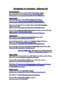
B. The income concept The income concept used for the analysis in sections II through IV is that of annual family income, adjusted for family size (the adjustment procedure is discussed in the following section). Total gross income of a family is defined as market income plus public social transfers and private tcansfers such as child alimony. Market income includes earnings, property income in cash, occupational and private pensions. Disposable income is defined as gross income minus income tax and compulsory social security contributions. Figure 1 illustrates the relations between the different aggregates4 All income aggregates refer to money income, including near-cash income elements such as food stamps. This means, that any income in kind - particularly imputed money values for education, health, housing, care and household production - is excluded from the estimates. An analysis of seven OECD countries included in the LIS data base suggests that imputed values for education and health constitute between 13 per cent (United States, Germany) and 22 per cent (Sweden, United Kingdom) of disposable income (Smeeding ef a/., 1993). In all countries, the percentage of these incomes in kind is particularly high for nonaged single parents and families with children. Preliminary estimates of money values for non-market household production (Chadeau, 1992) show that these are high relative to GDP and suggest that indicators of income inequality would be reduced, if imputed values of income derived from household production were added to money incomes. Also, the complex issue of intra-family transfers cannot be tackled sufficiently with the available micro data. Commonly, it is assumed that ~ needs to be taken into individuals share total family resources e q ~ a l l y .This account when interpreting the results in sections 11, Ill and IV.

184

!

Figure 1. Structure of income variables

__

__

Gross wage and salaries

+ +

Farm self-employment income Non-farm self-employmentincome

+

:---Earnings

____

Factor income

__.

Cash property income

+

Sick pay

+

Accident pay

+

Disability pay

+ +

Social retirement benefits Child or family allowances

Social insurance transfers

+ Unemployment compensation +

Social transfers

Maternity pay

+

Miiitary/veteran/war benefits

+

Other social insurance

+

Means tested cash benefits

+

Means-tested income

r

Near cash benefits

+

Private pensions

.___ Occupational _

+

pensions

Public sector pensions

+

Alimony or child support

+ +

;----- Private transfers

Other regular private income

Other cash income

+

=Total gross income

Market income = Factor income + occupational pensions. Disposable income = Gross income - mandatory contributions for self-employed - income tax - mandatory employee contributions.

185

C. Adjustment of incomes for family size and definition of the reference population One can assume that, due to economies of scale, the needs of a family for resources grow with each additional member, but not proportionally. With the help of equivalence scales, each family type in the population is assigned a value in proportion to its needs. When family size is used as the sole determinant for adjustment: equivalence scales can be represented by one single parameter, the equivalence elasticity, i.e. the power by which needs increase as family size increases: N = 3, or

where e: equivalence elasticity N: economic need (proxied by disposable income/economic wellbeing) S: family size

The equivalence elasticity, e, can thus range from 0 (when unadjusted family disposable income is taken as the income measure) to 1 (when per capita family income is used). The smaller the value for e, the higher are the assumed economies of scale. In selecting a particular equivalence scale, it is important to be aware of the potential effects on the size of the low-income population, its composition, and the relative positions of countries in international comparisons. The research of Buhmann et a/. (1988) suggests that, in general, adjusted low-income rates are lower at higher elasticities.’ As for the composition of the low-income population, almost by definition, the larger the elasticity, the greater the share of large families (thus children) among the low-income population and the smaller the share of single persons (thus elderly) and older married couples. However, at the same time the ranking of countries in cross-country comparison is, in general, not affected by the use of different equivalence scales. Buhmann e t a / . (1988) and OECD (1994) review a large inventory of some 50 equivalence scales. Scales derived by self-assessment from household surveys imply relatively low values for e (between 0.2 and 0.4) and typically underestimate the costs of additional family members. “Statistical” equivalence scales - for example the scale suggested in OECD Social Indicators (1982)* have relatively high elasticities (around 0.7). As the following analysis will focus on public policy actions to alleviate poverty, a “policy-based” equivalence scale with an elasticity of 0.55 will be used to adjust family incomes. Such a scale represents values which are inherent in many social programmes of OECD Member countries, and also comes quite close to equivalence values found in several surveys on household consumption expenditures.

186

Non-elderly families have been chosen as the reference population in sections II and 111. These are defined as families in which the head is aged under 60. Unfortunately, data for Italy and the Netherlands are only available on a household rather than a family basis. Also, a particular unit definition for Sweden based on tax units is likely to result in overestimates of low incomes for this c ~ u n t r y For .~ considerations on child poverty in section IV, estimates are based on the reference population of children. This means that low-income rates are calculated by defining the number of children living in low-income families with respect to the total population of children. Children are defined according to the classification of the LIS data sets, i,e. as unmarried persons under the age of 18 living in the family. D. The measurement of low incomes and poverty 1.

Head-count ratios, low-income gap and low-income distribution

A commonly used low-income measure is the head-count ratio, i.e. the number of persons or families with low incomes as a proportion of the total population. This so-called “low-income rate” is therefore defined as:

LIR = where q = number of units having incomes below z n = total population z = low-income threshold The low-income rate provides useful information on the incidence of lowincome situations but does not capture the intensity of such situations. For example, poverty would be considered more serious in a country where the average income of the same number of poor falls further below a given cut-off line. Comparing low-income rates between countries without paying due attention to the income levels of the low-income population may therefore be insufficient for policy considerations. A common indicator of this intensity is the average lowincome gap (ALG), which is defined as the difference between the average income of the low-income population and the low-income line, as a percentage of that line:

where q = number of persons having incomes below z z = low-income threshold

y, = income of the ith individual of the low-income population

vq = average income of the low-income population 187

However, a third aspect of low income must also be taken into account, namely the fact that some low-income families are poorer or richer than others. The low-income rate says nothing about the distribution of incomes among lowincome families. This aspect of poverty is also ignored by the low-income gap as it measures the distance below the average low income and the low-income line and is therefore insensitive to redistribution among the low-income population. A summary statistic used to characterise the distribution of incomes is the Gini coefficient (G) which lies between 0 - when all incomes are distributed equally, and 1 - when there is perfect inequaIity.’o The literature contains various methods to express the Gini coefficient; a common formula is:

where the y, are ranked in ascending order by their subscripts. Summarising these different aspects, the extent of poverty in a country depends on: i) the number (or fraction) of persons/families below a defined low-income standard, as measured by the low-income rate (LIR); ii) the severity of the low-income situation which can be proxied by the average low-income gap (ALG); and iii) the distribution of income among the low-income population, proxied by, for instance, the Gini coefficient. 2.

,

Synthetic indicators: the Sen poverty index

Sen (1976) developed an approach to combine these three elements into a single indicator of poverty for a given poverty line. His proposed measure consists of the head-count ratio multiplied by the sum of the income-gap ratio and the Gini coefficient of the poor weighted by the ratio of the mean income of the poor to the poverty-line income level. The Sen Index is thus defined as: S = LIR * (ALG +

* GP)= LIR * [ALG + (1 - ALG) * Gp] z where LIR = low-income rate (head-count ratio) ALG = average low-income gap (income shortfall) y, = mean income of the poor z = poverty line G, = Gini coefficient of income inequality among the poor In short, the Sen index can be interpreted as a weighted sum of poverty gaps of the poor. The values for the Sen index lie in the closed interval [0,1], with S = 0 if everyone has an income above the poverty line, and S = 1 if everyone is below the low-income level and the income distribution is characterised by perfect inequality or else, if everyone has zero income. Like many summary statistics of

188

income inequality, the Sen index assumes an ordinal approach to comparisons of welfare (for a discussion of the analytical foundations of the Sen index, see Forster, 1994: 38f). The Sen index is equal to the low-income rate multiplied by the average lowincome gap (LIR * ALG)” in the case of perfect income equality among the lowincome population, and equal to the low-income rate (LIR) in the case of perfect inequality: S = LIR * ALG for G, = 0 S = LIR for G, = 1 In the first case, i.e. when all the poor have the same income, the lower the income of the poor, the closer will S be to LIR; and the larger the proportion of the poor, the closer will S be to ALG. The Sen index is a useful measure for cross-country comparisons of poverty, because it combines the incidence, the intensity and the distribution of low incomes in a single indicator. Traditional measures such as the low-income rate and the average low-income gap fail to capture one or the other of these elements of poverty and provide therefore an incomplete picture when comparing poverty levels across countries. This is particularly important for the analysis of the effects of net taxes and transfers on low-income groups across countries since these might result in different (sometimes opposite) changes for one or the other components of poverty.

II. NON-ELDERLY FAMILIES: THE IMPACT OF NET TRANSFERS ON LOW INCOMES A.

Low-income rates

The percentage of families below a certain income threshold provides a basic indicator of the importance of low incomes among non-elderly families. It should be stressed that a low-income threshold z does not represent a break-even point below which a person (or family) suddenly becomes poor. Instead, low-income lines serve to define several classes of low income. Table 1 presents such lowincome classes, from 20 per cent to 70 per cent of the median disposable income. The estimates refer to post-tax and transfer incomes of non-elderly families. Three groups of countries can be distinguished in Table 1: i) Australia, Canada and the United States (especially at the top end of the scale) all have low-income rates well above the average in all income segments. ii) Some continental European countries - Austria, Belgium, Germany, Luxembourg and the Netherlands - are at the bottom in all of the segments. Within this grouping, Luxembourg has the lowest values for the

189

Table 1. Cumulative percentages of non-elderly families with low incomes Per cent of median income

Australia 85/86 Austria 87

Belgium 85 Canada 87 France 84 Germany 84/85 Ireland 87 Italy 86 Luxembourg 85 Netherlands 87 Noway 86 Sweden 87 United Kingdom 86 United States 86 Average (unweighted)

20

30

40

50

60

70

2.2 0.4 0.7 2.5 1.7 0.4 2.2 0.8 0.4 0.8 1.4 1.8 1.8 4.0 1.5

4.4 1.2 1.1 4.7 3.4 1.6 3.4 2.7 0.8 1.2 3.3 4.1 3.0 8.8 3.1

8.9 3.0 2.3 10.5 5.2 3.8 5.5 5.6 1.7 2.4 4.7 6.9 5.6 13.9 5.7

15.7 6.2 5.4 15.4 8.9 8.5 15.7 10.1 4.5 4.7 7.8 10.6 12.4 18.7 10.3

21.3 11.2 11.6 21.l 15.0 14.5 23.4 17.3 10.6 11.3 12.3 16.1 20.6 24.4 16.5

27.3 17.6 21.3 27.8 23.1 21.9 30.3 27.3 20.1 20.7 19.4 21.6 28.1 30.6 24.1

Notes: Income concept used is disposable income adjusted for family size. using an equivalence scale with an elasticity of 0.55. Non-eiderly families: families headed by a person aged less than 60. Source: LIS micro data base.

very low income segments (below 20 and 30 per cent); this means that the poor population in this country is concentrated towards higher cut-off lines (50 and 60 per cent). In Germany, the poor population seems to be more equally distributed within the segments. iii) The remaining European countries - France, Ireland, Italy, Norway, Sweden and the United Kingdom - have low-income rates close to the average, but there are different patterns according to the segment. In the 50 to 70 per cent range, for instance, France and Noway have lowincome rates significantly below the average, whereas Italy and Ireland have rates close to those of the first country group. Table 1 also reveals some country-specific patterns: some countries (Italy) have below-average rates in the lowest income segment (below 20 per cent) but above-average rates when moving to higher low-income segments. Other countries (Noway, Sweden) show the opposite picture. Both Ireland and the United Kingdom have above-average rates for the poorest population, average or belowaverage rates for the segments often defined as the “core” of the poor (below 40 per cent), and above-average rates for the population “near poverty” (60 and 70 per cent segment). In the following, poverty among non-elderly families is first measured with respect to their market incomes and then compared to poverty measured in terms of disposable incomes. This allows an analysis of the combined effect of income

190

Low incomes and public expenditures on social transfers There is widespread agreement that public spending influences the level as well as the composition of poverty. However, the magnitude of this influence, sometimes also its direction, are controversial issues. In some OECD countries, there is an increasing concern about persistent dependency of low-income families on public transfers. By providing basic security in the case of old-age, sickness, disability, unemployment and family situation, the welfare state tries to limit the extent of poverty. There are, however, substantive differences amongst countries in the extent and the generosity of the public social sector. Some studies analyse the relationship between the size of the welfare state and cross-national variations in poverty. Gustafsson and Uusilato (1989: 6), for example, claim that “the bigger the welfare state the smaller is the poverty rate.” This hypothesis can be illustrated by a simple cross-section regression for the 14 countries included in this study. The independent variable, the size of the welfare state, is proxied by total public expenditures on pensions, unemployment, family and other allowances as a share of GDP. Health and education expenditures are not included since they constitute in-kind transfers and the poverty estimates are based on disposable incomes. The dependent variable is the low

Figure A l . Low-income rates and public social transfer expenditures

Low-income rate

20

l6 14

Low-Income rate

,

, 20

1

0

b Unlled Slates

France

.t

0 Sweden

Luxembourg 0

. .Js 9

.

6

8

10

12

14

16

18

20

22

24

26

28-

Public lransler expendllures In per cent of GDP

Nole: Low-income rate defined as percentage of persons in families with incomes below 50 per cent of the median adjusted income.

Source: LIS micro data base; OECD Social data base.

(continued on next page)

191

(continued)

-income rate (50 percent level) for the entire population (i.e. including elderly persons, as old-age pensions are also included in total public expenditures on social transfers). Figure A . l shows that there is a significant negative correlation between these two variables across countries. The regression equation is: LIR = 20.4 - 0.66 * SOC with

R2 = 0.667, and standard error of coefficient = 0.13

When the dependent variable is defined at the 60 percent income level, the correlation is even stronger:

LIR = 28.5 - 0.76 SOC with R2 = 0.761, and standard error of coefficient = 0.15 In both cases, three groups of countries can be distinguished: the United States and Australia both have the highest low-income rate and the lowest social spending as a share of GDP. On the other hand, the Scandinavian and continental European countries (except Italy) have relatively low poverty rates and high public transfer expenditures. Within this group,. the difference between the two Scandinavian countries with respect to public transfers is noteworthy. Canada, the United Kingdom, Ireland and Italy lie in between. 9

taxes and transfers on low income.12 A separate assessment of the effects of social transfers alone is not very meaningful, as a significant decrease in poverty for a certain population group due to social transfers may partly be offset by a relatively high burden of personal taxation for the same group. In some countries this is the case, for example, for low-income families with many children. The estimates for two of the eleven countries reported below have to be treated with special care: the results for France (before net transfers) are not fully comparable with the other countries, as social security contributions (unlike the other countries) are not regarded as part of the personal income tax, and are therefore excluded. Also the results for Sweden are not fully comparable with those of other countries, as explained in section I. For reasons of sensitivity testing, poverty estimates for three low-income bands are presented: 40, 50 and 60 per cent below the median income level.

8 . Sen indices and components of low incomes As set out in section I, overall poverty as measured by the Sen index can be decomposed into incidence, intensity and income inequality. The respective values, referring to disposable incomes, are shown in the first three columns of Table 2. When analysing the results for the resulting Sen indices shown in

192

Table 2. Sen poverty measure and its components for disposable incomes, percentage change and relative contribution of components after accounting for net transfers Non-elderly families below 50 per cent of median income Indicators for low disposable incomes Low-income rate LIR

A

W

0

Relative contribution of components

(4)

Reduction in Sen index (percentage change) (5)

Low-income rate LIR (6)

Low-income gap ALG

(7)

GP (8)

Low-income

Gini (poor)

(1)

gap ALG (2)

GP (3)

Australia 85/86 Austria 87 Belgium 85 Canada 87 France 84 Germany 84/85 Ireland 87 Italy 86 Luxembourg 85 Netherlands 87 Noway 86 Sweden 87 United Kingdom 86 United States 86

15.7 6.2 5.4 15.4 8.9 8.5 15.7 10.1 4.5 4.7 7.8 10.6 12.4 18.7

30.7 24.0 25.0 33.2 33.3 23.2 24.9 27.3 22.4 28.8 35.5 41.0 27.6 39.5

0.1952 0.1187 0.1748 0.1890 0.2185 0.1340 0.1730 0.1616 0.1513 0.1971 0.2292 0.1485 0.1907 0.2326

6.94 2.05 2.06 7.05 4.26 2.84 5.94 3.94 1.54 2.01 3.93 5.28 5.13 10.02

47.9 n.a. 78.1 41.4 60.7 71.O 70.0 n.a. n.a. 82.8 53.7 60.2 72.1 22.8

25% n.a. 91% 43% 86% 43% 51% n.a. n.a. 73% 57% 62% 57% 17%

44% n.a. 4% 33% 8% 32% 31% n.a. ma. 19% 28% 17% 25% 43%

31% n.a. 6% 24% 5% 25% 18% n.a. n.a. 8% 15% 22% 17% 40%

Average (unweightec

10.3

29.7

0.1796

4.50

60.1

55%

26%

19%

Sen index S

Nofes: Income adjusted with an equivalence elasticity of 0.55. LIR. ALG,and Sen index multl Relative contributions estimated by linear approximation of Sen index (explanation rate! . . 85 per cent). Definitions and methods of indicators: see Section I. Source: LIS micro data base.

Gini (poor)

ed bv 100. bove' 92 per cent, except for Ireland. Netherlands and Sweden:

column (4), the cross-country patterns derived e rlier with the use of the lowincome rate become more accentuated. Five groups of countries can be distinguished: i) first, the European countries Austria, Belgium, Germany, Luxembourg and the Netherlands with Sen indices significantly below the average; ii) a second group of European countries - Noway, France and Italy which have indices just below the average; iii) third, the remaining European countries - Sweden, Ireland and the United Kingdom - with indices just above the average; iv) fourth, Australia and Canada with poverty indices above the cross-country average; v) fifth, the United States has very high low-income indicators which result in a Sen index that is more than double the average of all 14 countries. Looking at its decomposition, it can be seen that the high rates of the fourth country group are due mainly to the high incidence of low incomes (expressed in the low-income rate); the intensity and distribution of low income in this group are closer to the average of all This contrasts in particular with the case of Norway, which has a low-income intensity and distribution patterns well above the average but below-average low-income incidence, which results in a relatively low Sen index. To a lesser degree, the same pattern can be found for the Netherlands and France. Another particular case is Ireland, with high low-income incidence but well below-average intensity and inequality among the poor; the net result is a Sen index which is not that much in excess of the sample average. Figure 2 traces values for Sen indices related to market income on the horizontal axis and Sen indices, once allowance is made for taxes and transfers, on the vertical axis. The results refer to the 50 per cent low-income cut-off line. It can readily be seen that poverty is reduced in all countries after accounting for net transfers: all country points are situated below the 45O-line (the "line of no change"). This also holds true for the 40 per cent and 60 per cent low-income segments and the two specific demographic groups studied in section 111, as will be seen below. This means, ceferis paribus, that the tadtransfer systems in all the countries studied succeeded in one of their prime aims: redistributing income towards vulnerable families. A second finding from Figure 2 is that the rank ordering of countries changes when allowance is made for taxes and transfers. A third general result is that the differences in the levels of Sen indices between low-poverty and high-poverty countries are larger after accounting for net transfers than before: the highest Sen index for market incomes is two-and-a-half times higher than the lowest, whilst the highest Sen index for disposable incomes is five times higher. Both findings imply that poverty is reduced in some countries more than in others by workings of the tax and transfer system. The absolute magnitude of poverty reduction can be seen as the vertical distance between the 45O-line and the country point. High reduction rates for Sen poverty indices are observed for the following countries: the Netherlands,

194

Figure 2, Sen index before and after accounting for net transfers Non-elderly families Sen index aller taxes and transfers

Sen index aller taxes and transfers

20

-

18

-

16

-

14

-

12

-

10

-

8 -

6 -

4 -

2

Belgium 6

2

2

0 Nelherlands

I

I

I

I

I

4

6

8

10

12

,

I

14

I

I

I

16

18

20

Sen index before taxes and transfers

Notes: Sen indices at the 50 per cent cut-otf level. Average: unweighted country sample average. Source: LIS micro data base.

Belgium, the United Kingdom, Germany and Ireland. The smallest reduction is in the United States. Looking at the absolute values of S for market incomes, it can be seen that poverty is highest in Ireland and the United Kingdom, and lowest in Norway, Belgium, and Germany. Once allowance is made for taxes and transfers, the

195

United States, Canada and Australia have the highest values for S, and Belgium, the Netherlands and Germany have the lowest values. Ireland and the United Kingdom are outliers: combining the highest poverty levels across countries before net transfers and close to average after accounting for net transfers. The opposite holds for the United States: the Sen poverty index is close to the average before allowance is made for net transfers, but twice the average of all the countries under study after accounting for taxes and transfers.

C. Components of poverty reduction Column (5) in Table 2 shows the percentage change in the overall Sen index, when allowance is made for taxes and transfers. The overall effect of net transfers is to reduce poverty in all countries studied. The average reduction across the country sample is 60 per cent: from 23 per cent in the United States up to around 80 per cent in Belgium and the Netherlands. What components play the leading role in lowering the Sen index? The identification of the predominant component provides information about the extent of targeting in the different tadtransfer systems. If, for example, net transfers result in a reduction of the low-income gap and the income inequality among the poor but not in a reduction of the low-income rate, this may indicate a certain targeting to the poorest sections of the population. If, on the other hand, the lowincome rate decreases at the same time as intensity and income inequality among the poor increase, this may suggest that net transfers have mainly been allocated to the better-off among the poor. The evidence from the LIS data sets summarised in Tables 2 and 3 suggests that targeting of net transfers to the poorest segments seems to be strongest in Australia, Canada and the United States and, to a lesser degree, in Germany, Ireland, Norway and the United Kingdom. There is no clear pattern to be observed for the remaining countries. Columns (6), (7) and (8) in Table 2 give estimates for the relative contribution of the three components which can be attributed to the reduction in overall poverty.14On average, at the 50 per cent cut-off level, the reduction of low-income incidence, i.e. in the number of poor, accounts for 55 per cent of the reduction in overall poverty. About one-quarter can be attributed to the reduction in lowincome intensity, and the remaining fifth to the reduction in income inequality among the poor. There are, however, substantial differences across the countries studied. Only in two countries - Australia and the United States - is the contribution of both low-income intensity and inequality to the reduction of overall poverty higher than that of low-income incidence: the reduction in the number of poor only accounts for 17 per cent (United States) and 25 per cent (Australia) of the overall reduction in poverty, when allowance is made for net transfers. On the other hand, in two European countries - Belgium and France - about nine-tenths of the poverty reduction due to net transfers can be attributed to the change in the

196

Table 3. Percentage change of Sen poverty measure and its components after accounting for net transfers Non-elderly families Market Income = 100

Australia 85/86

< 40% of median < 50% of median c 60% of median

Belgium 85

< 40% of median < 50% of median < 60% of median

Canada 87

< 40% of median < 50% of median < 60% of median

France 84

< 40% of < 50% of < 60% of < 40% of

Germany 84/85

Ireland 87

Netherlands 87

Noway 86

Sweden 87

United Kingdom 86

United States 86

Average

,

Low-income

Low-income

rate LIR

gap ALG

Gini (poor) GP

Sen index

S

median median median median < 50% of median < 60% of median < 40% of median < 50% of median < 60% of median < 40% of median < 50% of median < 60% of median < 40% of median < 50% of median < 60% of median < 40% of median < 50% of median < 60% of median < 40% of median < 50% of median < 60% of median < 40% of median < 50% of median < 60% of median

58.2 89.2 103.9 14.4 23.8 38.8 66.5 81 .I 93.0 35.9 43.2 55.1 35.5 68.5 99.3 23.3 59.7 78.3 13.3 24.9 57.4 45.6 66.1 84.8 44.5 57.6 72.5 25.9 51.7 76.9 86.9 96.4 105.6

55.1 53.9 63.6 101.7 94.0 88.8 64.7 71.3 74.0 95.7 89.6 80.8 36.4 38.9 44.3 71.4 43.5 51.1 72.3 62.8 45.9 74.7 64.6 75.4 74.0 75.5 77.2 63.8 48.3 50.2 72.3 80.3 83.2

52.2 44.8 48.0 93.5 87.0 70.4 58.5 60.2 64.2 87.1 88.6 82.5 27.5 27.7 31.4 66.2 40.9 39.3 87.9 66.5 47.9 62.9 61.I 57.6 35.2 38.4 40.8 55.5 42.1 39.4 61.5 66.8 71.4

36.5 52.1 67.1 14.2 21.9 32.2 45.2 58.6 69.9 33.7 39.3 46.3 14.7 29.0 46.1 17.9 30.0 42.1 10.8 17.2 29.8 34.9 46.3 63.2 29.9 39.8 51 .I 18.0 27.9 41 .O 64.4 77.2 87.7

40% of median < 50% of median < 60% of median

40.9 60.2 78.7

71.1 65.7 66.8

62.6 56.7 53.9

29.1 39.9 52.4